k-Means Clustering
Math 123: Mathematical Aspects of Data Analysis – Fall 2026
Where we are
Last time we ranked the vertices of a graph with PageRank. Today we return to a point cloud \(\bfx_1,\ldots,\bfx_n\in\Rbb^d\), stacked as the rows of a data matrix \(\bfX\), and ask for groups instead of directions: can the points be split into a few clusters of similar observations? This is Section 5.3 of the textbook.
Throughout, \(\mathbf{1}\) is the all-ones vector (with its length as a subscript when it matters), \(\bfe_\ell\) is the \(\ell\)-th standard basis vector, and \([n]=\{1,\ldots,n\}\).
Clustering
Clustering is the task of splitting data into groups, or clusters, so that points in the same group are similar and points in different groups are not. “Similar” can mean close in Euclidean distance, for points in \(\Rbb^d\), or well connected, for the vertices of a graph. Unlike regression, there is no response \(\bfy\) telling us the right answer: clustering is unsupervised. That makes it both useful (no labels needed) and slippery (what is the right answer?).
We start with points in \(\Rbb^d\) and the most popular clustering method of all.
The k-means problem
Fix data points \(\bfx_1,\ldots,\bfx_n\in\Rbb^d\) and a number of clusters \(k\leq n\). A \(k\)-partition of the data is a split of \([n]\) into disjoint non-empty sets \(S_1,\ldots,S_k\) whose union is \([n]\). For a non-empty \(S\subseteq[n]\), write \[ \bar{\bfx}_S=\frac1{|S|}\sum_{i\in S}\bfx_i \] for the mean of the points in \(S\), and \(\bar{\bfx}=\bar{\bfx}_{[n]}\) for the overall mean.
Each point pays the squared distance to the center of its own cluster. There are only finitely many \(k\)-partitions, so the minimum exists, but there are a lot of them (roughly \(k^n/k!\) for large \(n\)), so trying them all is hopeless.
The cost is a sum of two kinds of choices: the partition, and the centers. Each is easy to optimize when the other is held fixed. For the centers, we need one identity that has already appeared twice in this course.
Proof. Write \(\bfx_i-\bfmu=(\bfx_i-\bar{\bfx}_S)+(\bar{\bfx}_S-\bfmu)\) and expand the square: \[ \sum_{i\in S}\|\bfx_i-\bfmu\|_2^2 =\sum_{i\in S}\|\bfx_i-\bar{\bfx}_S\|_2^2 +2(\bar{\bfx}_S-\bfmu)^\top\sum_{i\in S}(\bfx_i-\bar{\bfx}_S) +|S|\,\|\bar{\bfx}_S-\bfmu\|_2^2. \] The middle sum is \(\sum_{i\in S}\bfx_i-|S|\bar{\bfx}_S=\mathbf{0}\) by the definition of the mean. The last term is non-negative and vanishes only when \(\bfmu=\bar{\bfx}_S\).
This is the bias–variance decomposition once more, with an average over \(S\) in place of an expectation: the mean squared distance to \(\bfmu\) is the spread around the mean plus the squared distance from the mean to \(\bfmu\). For \(d=1\) it is also fitting a constant by least squares.
Proof. For part 1, the cost is a sum of \(k\) separate terms, the \(\ell\)-th depending only on \(\bfmu_\ell\); minimize each one by Lemma 1. For part 2, point \(i\in S_\ell\) contributes \(\|\bfx_i-\bfmu_\ell\|_2^2\geq\min_m\|\bfx_i-\bfmu_m\|_2^2\), with equality exactly when \(\bfmu_\ell\) is a nearest center. For the last claim, minimizing over partitions and centers jointly is the same as first minimizing over centers for each fixed partition, which by part 1 leaves \(\operatorname{WCSS}\).
So \(k\)-means looks for the partition whose clusters are as tight as possible. There is another useful way to express that tightness.
Proof. Apply Lemma 1 to each \(S_\ell\) with \(\bfmu=\bar{\bfx}\), and sum over \(\ell\).
The total on the left is \(n\) times the total variance. So, just as PCA splits the total variance into a retained part and a lost part, \(k\)-means splits it into a part explained by the clusters (the spread of the cluster means) and a part left inside the clusters. Tight clusters and well-separated clusters are the same goal.
Lloyd’s algorithm
Proposition 1 suggests alternating between the two easy problems. This is Lloyd’s algorithm, often simply called “the \(k\)-means algorithm”.
Each iteration costs \(O(nkd)\): compute \(nk\) distances in \(\Rbb^d\), then \(k\) averages.
Proof. Allow empty clusters for the moment, and for an assignment \(c:[n]\to[k]\) and centers \(\bfmu_1,\ldots,\bfmu_k\) write \[ J(c,\bfmu)=\sum_{i=1}^n\|\bfx_i-\bfmu_{c(i)}\|_2^2, \qquad F(c)=\min_{\bfmu}J(c,\bfmu). \] By Lemma 1, the minimum defining \(F(c)\) is attained by putting each center of a non-empty cluster at the cluster mean; centers of empty clusters do not appear in \(J\) at all. So after every update step, \(J_t=F(c_t)\), where \(c_t\) is the assignment in force during that step.
Now suppose the next assignment step produces \(c_{t+1}\neq c_t\), with the centers \(\bfmu^{(t)}\) from update step \(t\). A point changes label only when its new center is strictly closer (ties keep the old label), and no point gets farther from its center, so \[ J(c_{t+1},\bfmu^{(t)})<J(c_t,\bfmu^{(t)})=J_t. \] The update step then gives \(J_{t+1}=F(c_{t+1})\leq J(c_{t+1},\bfmu^{(t)})\). So \(F(c_{t+1})<F(c_t)\), proving part 1.
Since \(F\) strictly decreases along the sequence of assignments visited, no assignment can appear twice, and there are \(k^n\) maps \([n]\to[k]\); this is part 2. At termination the assignment did not change, so every point is at a nearest center, and the last update step put every center of a non-empty cluster at its mean; this is part 3.
Two caveats. First, the \(k^n\) bound is astronomically pessimistic; in practice Lloyd’s algorithm usually stops after a few dozen iterations. Second, and more importantly, stopping is not the same as solving the problem. Part 3 describes a configuration that neither step can improve, which is a kind of local minimum, and these can be terrible.
This is not just bad luck with one algorithm. The \(k\)-means problem is NP-hard, even for \(k=2\) (when the dimension \(d\) is allowed to grow), so (assuming \(\mathrm{P}\neq\mathrm{NP}\)) no efficient algorithm solves every instance exactly. In practice we live with local search and use good starting points.
Initialization: k-means++
Since the outcome depends on the starting centers, two practical remedies are standard.
- Restarts. Run Lloyd’s algorithm from several random initializations and keep the result with the smallest cost.
- Careful seeding. Choose initial centers that are spread out, so that no two start in the same true cluster.
Points far from the current centers are likely to become new centers, and points already covered (with \(D(\bfx_i)=0\)) are never picked again. Arthur and Vassilvitskii (Arthur and Vassilvitskii 2007) proved that the seeding alone already has expected cost at most \(8(\ln k+2)\operatorname{opt}_k\), and by Theorem 2 the Lloyd iterations afterwards can only lower it. In Example 1, if the first center is \(\bfx_1\), then the squared distances to the other corners are \(1\), \(L^2\), and \(L^2+1\), so the second center lands on the far side of the rectangle with probability \((2L^2+1)/(2L^2+2)\). From such a start, Lloyd’s algorithm finds the left/right optimum (check this!), so k-means++ avoids the bad fixed point with probability tending to \(1\) as \(L\) grows. The guarantee is only in expectation, though, so restarts are still worthwhile. See the example k-Means: A Bad Fixed Point for pictures of both fixed points, their basins of attraction, and a simulation of both seedings.
- In scikit-learn,
KMeans(n_clusters=k, init="k-means++", n_init=10).fit(X)runs k-means++ followed by Lloyd’s algorithm from \(10\) seeds and keeps the best. The fitted object haslabels_(the assignment),cluster_centers_, andinertia_(the final cost). - The cost uses Euclidean distance with all features on an equal footing, so, as with ridge regression, the answer depends on the units. Standardize the features first unless they share a natural scale.
- Lloyd’s algorithm in NumPy is short; writing it once yourself is a good way to understand it.
import numpy as np

def lloyd(X, centers, max_iter=100):
    centers = np.array(centers, dtype=float)  # copy, so the caller's array is untouched
    labels = None
    for _ in range(max_iter):
        dists = ((X[:, None, :] - centers[None, :, :]) ** 2).sum(axis=2)  # (n, k)
        new_labels = dists.argmin(axis=1)
        if labels is not None and np.array_equal(new_labels, labels):
            break
        labels = new_labels
        for l in range(len(centers)):
            if np.any(labels == l):
                centers[l] = X[labels == l].mean(axis=0)
    cost = ((X - centers[labels]) ** 2).sum()
    return labels, centers, cost
(Here argmin breaks ties by the smallest index rather than by keeping the old label, which is harmless in practice since exact ties are rare.)
k-means as a matrix factorization
There is a compact way to write the \(k\)-means cost that connects it to everything we did with the SVD and least squares. Encode a \(k\)-partition by its membership matrix \(\bfH\in\{0,1\}^{n\times k}\), with \(H_{i\ell}=1\) if \(i\in S_\ell\) and \(0\) otherwise, so each row of \(\bfH\) is a standard basis vector \(\bfe_\ell^\top\). Stack the centers as the rows of \(\bfM\in\Rbb^{k\times d}\). Then row \(i\) of \(\bfH\bfM\) is \(\bfmu_\ell^\top\) for the cluster \(\ell\) containing \(i\), so \[ \operatorname{cost}(S_1,\ldots,S_k;\bfmu_1,\ldots,\bfmu_k)=\|\bfX-\bfH\bfM\|_F^2. \] \(k\)-means approximates the data matrix by a product \(\bfH\bfM\) in which \(\bfH\) is constrained to be a membership matrix.
Fixing \(\bfH\) turns this into an ordinary least squares problem in \(\bfM\), one column (feature) at a time. The columns of \(\bfH\) are the indicator vectors of the clusters, so they are orthogonal and \(\bfH^\top\bfH=\operatorname{diag}(|S_1|,\ldots,|S_k|)\) is invertible. The normal equations give \[ \bfM=(\bfH^\top\bfH)^{-1}\bfH^\top\bfX, \] whose \(\ell\)-th row is \(\frac1{|S_\ell|}\sum_{i\in S_\ell}\bfx_i^\top=\bar{\bfx}_{S_\ell}^\top\). The update step of Lloyd’s algorithm is a regression of each feature on the cluster indicators, that is, fitting one constant per cluster.
Without the constraint on \(\bfH\), the best approximation of \(\bfX\) by a product with \(k\) columns in the middle is the truncated SVD, by Eckart–Young. That gives a lower bound on what \(k\)-means can achieve.
Proof. Fix a \(k\)-partition with means \(\bfmu_\ell=\bar{\bfx}_{S_\ell}\), membership matrix \(\bfH\), and center matrix \(\bfM\). Since every row of \(\bfH\) sums to one, \(\bfH\mathbf{1}_k=\mathbf{1}_n\), and so \[ \bfX-\bfH\bfM=(\bfX-\mathbf{1}_n\bar{\bfx}^\top)-(\bfH\bfM-\bfH\mathbf{1}_k\bar{\bfx}^\top)=\bfX_c-\bfH\bfB, \qquad \bfB=\bfM-\mathbf{1}_k\bar{\bfx}^\top. \] The rows of \(\bfB\) are \((\bfmu_\ell-\bar{\bfx})^\top\), and they satisfy one linear relation with non-zero coefficients: \[ \sum_{\ell=1}^k|S_\ell|(\bfmu_\ell-\bar{\bfx})=\sum_{i=1}^n\bfx_i-n\bar{\bfx}=\mathbf{0}. \] So the \(k\) rows of \(\bfB\) are linearly dependent, \(\operatorname{rank}(\bfB)\leq k-1\), and therefore \(\operatorname{rank}(\bfH\bfB)\leq k-1\). By Eckart–Young in the Frobenius norm applied to \(\bfX_c\), \[ \operatorname{WCSS}(S_1,\ldots,S_k)=\|\bfX_c-\bfH\bfB\|_F^2\geq\min_{\operatorname{rank}(\bfC)\leq k-1}\|\bfX_c-\bfC\|_F^2=\sum_{j\geq k}\sigma_j^2. \] Minimize over partitions and use Proposition 1. For \(k=1\) there is only one partition, with \(\operatorname{opt}_1=\|\bfX_c\|_F^2=\sum_j\sigma_j^2\).
In words: the \(k\) cluster means, recentered, span at most a \((k-1)\)-dimensional subspace, so \(k\)-means can never beat PCA with \(k-1\) components. This is one reason why projecting the data onto its top few principal directions before running \(k\)-means is a common preprocessing step: it makes each iteration cheaper, and the directions it discards are ones along which the clusters cannot be very spread out anyway.
Remark (Relaxation). Replacing the hard combinatorial constraint “\(\bfH\) is a membership matrix” by a softer one that linear algebra can handle is called a relaxation. The relaxed problem is solved by eigenvectors or singular vectors, and its solution is then rounded back to a partition. This is the strategy of spectral clustering, coming up after we introduce graphs, applied to a graph instead of a point cloud.
Choosing k
So far \(k\) was given. Can we choose it by minimizing the cost?
Proof. See Homework 6, Problem 2.
This is the same trap as choosing \(\lambda\) by training error: the objective always prefers the most flexible model. Unlike in regression, there are no held-out labels to cross-validate against, so choosing \(k\) is genuinely a modeling decision. Common heuristics include:
- the elbow method: plot \(\operatorname{opt}_k\) (or the cost found by k-means++) against \(k\) and look for the point where adding clusters stops helping much;
- silhouette scores, which compare each point’s average distance to its own cluster with its average distance to the nearest other cluster;
- domain knowledge, which is often the best guide of all.
What k-means cannot do
Proof. Expanding both sides of \(\|\bfx-\bfmu_\ell\|_2^2\leq\|\bfx-\bfmu_m\|_2^2\), the \(\|\bfx\|_2^2\) terms cancel, leaving \[ 2(\bfmu_m-\bfmu_\ell)^\top\bfx\leq\|\bfmu_m\|_2^2-\|\bfmu_\ell\|_2^2, \] which is linear in \(\bfx\): a half-space. \(R_\ell\) is the intersection of these half-spaces over \(m\neq\ell\), and intersections of convex sets are convex.
The regions \(R_\ell\) are the Voronoi cells of the centers. By Theorem 2, the output of Lloyd’s algorithm assigns each point to a nearest center, so every cluster it produces is the set of data points lying in one convex cell (up to ties on the boundaries). Any two clusters are separated by a hyperplane.
Figure 1 shows the consequence. Round, well separated blobs are exactly what \(k\)-means is built for. Two concentric rings are obviously two clusters to the eye, but no hyperplane separates them, so \(k\)-means has no chance: it cuts the picture in half instead.
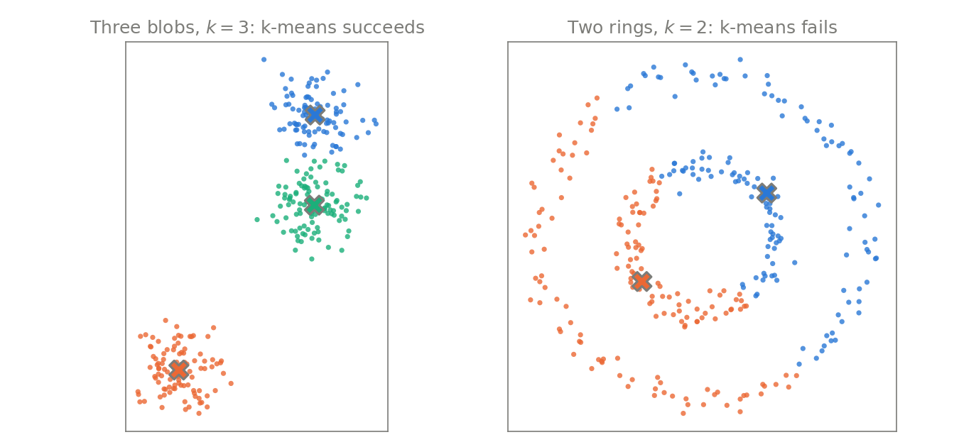
To summarize the limitations of \(k\)-means:
- the number of clusters \(k\) must be chosen in advance;
- the problem is NP-hard, and Lloyd’s algorithm only finds a local minimum;
- it needs points in \(\Rbb^d\) (though Homework 6, Problem 3 shows that pairwise distances are enough), and it depends on the scaling of the features;
- squared distances make it sensitive to outliers (replacing \(\|\cdot\|_2^2\) by \(\|\cdot\|_1\) gives the more robust \(k\)-medians, Exercise 5.5 of the textbook);
- its clusters are always convex.
Summary
\(k\)-means turned “find the groups” into the minimization of the within-cluster sum of squares, equivalently \(\min\|\bfX-\bfH\bfM\|_F^2\) over membership matrices \(\bfH\) and centers \(\bfM\). The problem is NP-hard, but Lloyd’s algorithm is a simple, monotone local search that always terminates (Theorem 2), though only at a local minimum, and k-means++ seeding gives it a good start. No partition can beat PCA with \(k-1\) components: \(\operatorname{opt}_k\geq\sum_{j\geq k}\sigma_j^2\) (Theorem 3). Its blind spot, non-convex clusters (Figure 1), is what motivates moving from point clouds to graphs next time.