The Basics of CQC Data

Math 123: Mathematical Aspects of Data Analysis – Fall 2026

Data as Vectors

Definition 1 (Observation and feature vector) An observation is one object being measured. A feature is one numerical measurement of that object.

If one observation has \(d\) real-valued features, its feature vector is \[ \bfx = \begin{pmatrix} x_1 \\ x_2 \\ \vdots \\ x_d \end{pmatrix} \in \Rbb^d. \]

The number \(d\) is the ambient dimension of the data representation.

Example 1 (Tabular observation) One student described by \[ \text{attendance},\quad \text{homework average},\quad \text{exam average},\quad \text{hours studied} \] is represented by one vector \(\bfx \in \Rbb^4\).

Example 2 (Image as a vector) A grayscale \(p \times q\) image is an array of pixel intensities. After choosing an ordering of the pixels, the same image is a vector in \(\Rbb^{pq}\).

An RGB image with three color channels is a vector in \(\Rbb^{3pq}\).

Example 3 (Document as a vector) Fix a vocabulary of \(d\) words. A document may be represented by \[ \bfx = (x_1,\ldots,x_d) \in \Rbb^d, \] where \(x_j\) records the count, frequency, or weighted frequency of word \(j\).

Data as Matrices

Definition 2 (Data matrix) A dataset with \(n\) observations and \(d\) features is stored as a matrix \[ \bfX = \begin{pmatrix} - & \bfx_1^\top & - \\ - & \bfx_2^\top & - \\ & \vdots & \\ - & \bfx_n^\top & - \end{pmatrix} \in \Rbb^{n \times d}. \]

Row \(i\) is observation \(\bfx_i^\top\). Column \(j\) is feature \(j\) across all observations.

TipRemark (Rows versus columns)

Remark (Rows versus columns). Two conventions:

• \(\bfX \in \Rbb^{n \times d}\): rows are observations, columns are features.
• \(\bfY \in \Rbb^{d \times n}\): columns are observations, rows are features.

These conventions are related by transposition: \(\bfY = \bfX^\top\).

Definition 3 (Point cloud) The rows of \(\bfX \in \Rbb^{n \times d}\) define a finite point cloud \[ \mathcal{X} = \{\bfx_1,\ldots,\bfx_n\} \subseteq \Rbb^d. \]

Data analysis tasks become geometric tasks on \(\mathcal{X}\):

• nearest-neighbor search,
• clustering,
• classification,
• regression,
• denoising,
• dimension reduction,
• outlier detection.

Big-Data is Messed Up

Definition 4 (Euclidean balls and cubes) For \(R>0\), the \(d\)-dimensional Euclidean ball of radius \(R\), centered at the origin, is \[ B_2^d(R) = \left\{\bfx \in \Rbb^d : \|\bfx\|_2 \le R\right\}. \]

The \(d\)-dimensional cube of side length \(R\), centered at the origin, is \[ C^d(R) = \left[-\frac{R}{2},\frac{R}{2}\right]^d. \]

Proposition 1 (Volumes of Euclidean balls and cubes) For \(R>0\), \[ \operatorname{vol}\!\left(B_2^d(R)\right) = \frac{\pi^{d/2}}{\Gamma(d/2+1)}R^d, \qquad \operatorname{vol}\!\left(C^d(R)\right) = R^d. \]

For fixed \(R\), Stirling’s approximation gives \[ \operatorname{vol}\!\left(B_2^d(R)\right) \sim \frac{1}{\sqrt{\pi d}} \left(\frac{2\pi e}{d}\right)^{d/2}R^d \qquad \text{as } d \to \infty. \] In particular, the volume of the unit ball \(B_2^d(1)\) vanishes as the dimension grows.

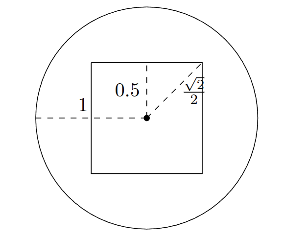
(a) The unit disk and centered unit square in two dimensions. Source: Bandeira et al. (n.d.), Section 2.1.1.

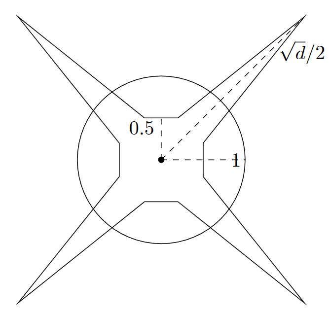
(b) A schematic comparison of the unit ball and centered unit cube in high dimension. Source: Bandeira et al. (n.d.), Section 2.1.1.

Figure 1: The Euclidean unit ball and centered unit cube in low and high dimensions.

Proposition 2 (Volume near the boundary) Let \(0 < \epsilon < 1\). Removing the outermost layer of thickness \(\epsilon\) from the unit ball leaves \(B_2^d(1-\epsilon)\), whose volume relative to the unit ball is \[ \frac{\operatorname{vol}\!\left(B_2^d(1-\epsilon)\right)} {\operatorname{vol}\!\left(B_2^d(1)\right)} = (1-\epsilon)^d. \] Consequently, for any fixed \(\epsilon>0\), this fraction tends to zero as \(d \to \infty\): almost all of the unit ball’s volume lies in its outermost \(\epsilon\) layer.

How do we interpret these facts? From Proposition 1 the unit ball covers proportionally less and less space as dimension grows larger. Many algorithms that ask, locally, what’s near me, will struggle in high dimensions precisely because of this fact! Moreover, although Proposition 1 indicates that the volume of the unit cube doesn’t vanish, note that the corners scale with dimensionality! While this may resolve our problem with vanishing volume, we have to understand that the d-dimensional cube is a tricky object to reason about because of the different scales. Finally, Proposition 2 indicates that nearly all the volume of a unit ball is contained near the boundary. Primarly, this is one of the key pieces of intuition for a concept known as concentration; that mass a high dimensions is often locally clustered.

Descent into Probability

Suppose we have a bunch of data, from the same ‘distribution’ \[ X_1,\ldots,X_n \] with a common mean \(\mu\). The average reading is \[ \overline{X} = \frac1n\sum_{i=1}^n X_i. \]

Our first probability question is the one that will guide both lectures:

Why should \(\overline{X}\) be close to \(\mu\), and how unlikely is it that it is not?

Random Variables, Distributions, and Events

Definition 5 (Random variable) A random variable is a numerical quantity whose value is determined by the outcome of a random experiment.

We write a random variable with a capital letter, such as \(X\), and a possible value with a lowercase letter, such as \(x\).

Definition 6 (Distribution and event) The distribution of \(X\) describes how probability is assigned to its possible values. For example, for a discrete random variable (a random variable taking discrete values), we may consider the probability that \(X\) takes on a random event. That’s typically written in the notation \[ \Pbb(X=x) \] for every possible value \(x\).

An event is a yes-or-no statement about the random outcome. For example, \[ \{X\ge 5\} \] is an event, and \(\Pbb(X\ge 5)\) is the probability that it occurs.

Example 4 (Three recurring examples)  

1. A Bernoulli random variable with parameter \(p\) has distribution \[ X= \begin{cases} 1, & \text{with probability }p,\\ 0, & \text{with probability }1-p. \end{cases} \] For example, you may consider a classifier determining whether an email is spam or not.

2. A Rademacher random variable is a random sign: \[ \Pbb(X=1)=\Pbb(X=-1)=\frac12. \] Seemingly arbitrary, but random signs appear in randomized linear algebra.

3. A standard Gaussian random variable, written \(X\sim N(0,1)\), is a continuous random variable with a symmetric bell-shaped distribution centered at \(0\). For continuous variables, probabilities are assigned to intervals by integrating over its associated density function. The standard Gaussian density is \[ \varphi(x) = \frac{1}{\sqrt{2\pi}}e^{-x^2/2}, \qquad x\in\Rbb. \] Therefore, if \(a\leq b\), then \[ \Pbb(a\leq X\leq b) = \int_a^b \varphi(x)\,dx = \Phi(b)-\Phi(a), \] where \(\Phi(t)=\int_{-\infty}^t \varphi(x)\,dx\) is the standard Gaussian cumulative distribution function.

Expectation

Definition 7 (Expectation) The expectation or mean of a discrete random variable is its probability-weighted average: \[ \Ebb[X] = \sum_x x\,\Pbb(X=x). \]

For a continuous random variable, the analogous definition uses an integral. If \(X\) has density \(f\), then \[ \Ebb[X] = \int_{-\infty}^{\infty}x f(x)\,dx. \] Note: Expectation describes the center of a distribution; it need not be a possible value of the random variable.

Example 5 (Bernoulli, Rademacher, and a die) If \(X\) is Bernoulli with parameter \(p\), then \[ \Ebb[X]=1\cdot p+0\cdot(1-p)=p. \]

If \(R\) is Rademacher, then \[ \Ebb[R]=1\cdot\frac12+(-1)\cdot\frac12=0. \]

If \(D\) is a fair six-sided die, then \[ \Ebb[D] = \frac{1+2+3+4+5+6}{6} = 3.5. \]

Proposition 3 (Linearity of expectation) For random variables \(X_1,\ldots,X_n\) and constants \(a_1,\ldots,a_n\), \[ \Ebb\!\left[\sum_{i=1}^n a_iX_i\right] = \sum_{i=1}^n a_i\Ebb[X_i], \] whenever the expectations exist.

Linearity of expectation does not require independence.

Example 6 (Expected number of successes) Let \(X_i\) equal \(1\) when trial \(i\) succeeds and \(0\) otherwise, and suppose each trial succeeds with probability \(p\). The number of successes is \[ S=X_1+\cdots+X_n. \] Whether or not the trials are independent, \[ \Ebb[S] = \sum_{i=1}^n\Ebb[X_i] = np. \]

Returning to repeated measurements with \(\Ebb[X_i]=\mu\), linearity gives \[ \Ebb[\overline{X}] = \frac1n\sum_{i=1}^n\Ebb[X_i] = \mu. \] Thus the average is centered at the right place.

References

Bandeira, Afonso, Amit Singer, and Thomas Strohmer. n.d. Mathematics of Data Science. https://people.math.ethz.ch/~abandeira/BandeiraSingerStrohmer-MDS-draft.pdf.