Linear Regression and Least Squares
Math 123: Mathematical Aspects of Data Analysis – Fall 2026
Recap
Last time we found the subspace that best fits a centered point cloud, and it turned out to be spanned by the top right singular vectors (best-fitting subspaces come from the SVD). We talked quite a bit about orthogonal projetions then. I’ll need some of those tools again; so to restate things:
Linear regression
Since 1958, the Mauna Loa Observatory in Hawaii has measured the concentration of carbon dioxide in the atmosphere. The plot of the monthly averages is called the Keeling curve, after Charles David Keeling, who started the measurements. This plot interesting, outside of the real-world implications, because it has some strange features. Note, it’s get steeper and there’s a yearly oscillation corresponding to the seasons. Suppose we have \(n\approx800\) monthly averages \(y_i\) (in parts per million), recorded at times \(t_i\) (in years since 1958). What concentration should we expect in, say, May 2030?
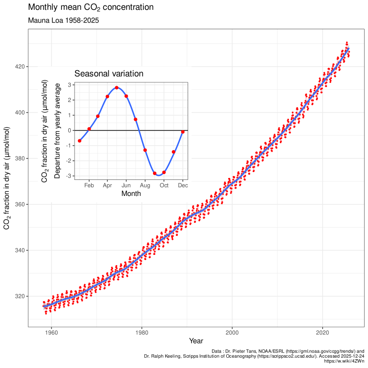
This curve is pretty far from linear! Just because this section is called linear regression doesn’t mean that we’re stuck fitting lines. A model can have non-linear output but still be linear in its tunable parameters. For example, \[ y\approx\theta_0+\theta_1t+\theta_2t^2+\theta_3\cos(2\pi t)+\theta_4\sin(2\pi t). \] This is a sample model for the above example that can work quite well! The quadratic captures the accelerating trend, and the cosine and sine together capture the yearly cycle, with the fit choosing both its size and the month of its peak. Note, the model is linear in the coefficients, not in \(t\)! Each observation simply contributes the features \((1,t_i,t_i^2,\cos(2\pi t_i),\sin(2\pi t_i))\) to our dataset. We will try to select the coefficients \(\theta_0,\ldots,\theta_4\) optimally from the data.
To allow a bias \(\theta_0\) (the intercept), we can augment \(\bfX\) to include a column of all ones \(\mathbf{1}\in\Rbb^n\).
In the Keeling example, \(\bfX\in\Rbb^{n\times5}\). Note, \(\bfX\) is not centered here, unlike the centered data matrix of the last two lectures.
Linear regression is used for two rather different purposes.
- Prediction. Given a new feature vector \(\bfx_{\text{new}}\), predict \(\widehat{y}_{\text{new}}=\bfx_{\text{new}}^\top\widehat{\bftheta}\), where \(\widehat{\bftheta}\) is our estimate of \(\bftheta\).
- Inference. Understand the relationship itself: which features matter, how much \(y\) changes when \(x_j\) does, and how confident we are in those answers.
Because of the noise \(\bfvarepsilon\), we cannot expect to recover \(\bftheta\) exactly. Moreover, we cannot expect \(\bfy\) to be perfectly modeled by \(\bfX\bftheta\) for any \(\bftheta\). So we need a way to measure how well a candidate \(\bftheta\) fits.
Why squares? We could just as well minimize the sum of absolute residuals \(\sum_i|y_i-\bfx_i^\top\bftheta|=\|\bfy-\bfX\bftheta\|_1\), or the worst residual \(\max_i|y_i-\bfx_i^\top\bftheta|=\|\bfy-\bfX\bftheta\|_\infty\). And, we could! But the squared loss has some nice advantages which ultimately result in why people use it as default.
- geometric: least squares corresponds to an orthogonal projection;
- computational: the minimizer is a linear system solve;
- statistics: under reasonable assumptions on \(\varepsilon\), least squares is the best estimator of its kind.
The idea is actually quite old (though maybe relatively new). Legendre published it in 1805 as a recipe for fitting orbits to astronomical data. Gauss published his version in 1809, claiming he had been using it since 1795 (surely this was hot drama at the time?). Gauss also supplied the first probabilistic justification, which we will see later.
Both least squares and PCA “fit features to a point cloud”, but least squares minimizes vertical distances while PCA minimizes perpendicular ones. See the example Regression Is Not PCA for a side-by-side comparison.
The geometry of least squares
Note! The vector \(\bfX\bftheta\) is the linear combination of the columns of \(\bfX\) with weights \(\theta_1,\ldots,\theta_d\). That is, it ranges over the column space \(\Ccal(\bfX)\subseteq\Rbb^n\). So minimizing \(\|\bfy-\bfX\bftheta\|_2\) over \(\bftheta\) is the same as finding the point of \(\Ccal(\bfX)\) closest to \(\bfy\). Yes, we have not finished beating things to death with orthogonal projections.
Proof. Every vector \(\bfX\bftheta\) lies in \(\Ccal(\bfX)\), so by Proposition 1, part 2, \[ \|\bfy-\bfX\bftheta\|_2\geq\|\bfy-\bfP\bfy\|_2, \] with equality if and only if \(\bfX\bftheta=\bfP\bfy\). Since \(\bfP\bfy\in\Ccal(\bfX)\), there is at least one \(\widehat{\bftheta}\) with \(\bfX\widehat{\bftheta}=\bfP\bfy\), and it attains the lower bound. This proves parts 1 and 2. Part 3 follows from part 2 and Proposition 1, part 1.
Note, the fitted values and residual are unique. Not necessarily the obtained \(\widehat{\bftheta}\).
The theorem says what \(\bfX\widehat{\bftheta}\) must be, but we still need a way to compute \(\widehat{\bftheta}\).
Proof. (\(\Rightarrow\)) By Theorem 1, part 3, the residual \(\widehat{\bfr}=\bfy-\bfX\widehat{\bftheta}\) is orthogonal to \(\Ccal(\bfX)\), and in particular to each column of \(\bfX\). The \(j\)-th entry of \(\bfX^\top\widehat{\bfr}\) is exactly the inner product of column \(j\) with \(\widehat{\bfr}\), so \(\bfX^\top\widehat{\bfr}=\mathbf{0}\).
(\(\Leftarrow\)) Suppose \(\bfX^\top(\bfy-\bfX\widehat{\bftheta})=\mathbf{0}\), and let \(\bftheta\in\Rbb^d\) be arbitrary. Split \[ \bfy-\bfX\bftheta =(\bfy-\bfX\widehat{\bftheta})+\bfX(\widehat{\bftheta}-\bftheta). \] The two pieces are orthogonal, because \[ \big(\bfX(\widehat{\bftheta}-\bftheta)\big)^\top(\bfy-\bfX\widehat{\bftheta}) =(\widehat{\bftheta}-\bftheta)^\top\bfX^\top(\bfy-\bfX\widehat{\bftheta}) =0. \] So by the Pythagorean theorem, \[ \|\bfy-\bfX\bftheta\|_2^2 =\|\bfy-\bfX\widehat{\bftheta}\|_2^2+\|\bfX(\widehat{\bftheta}-\bftheta)\|_2^2 \geq\|\bfy-\bfX\widehat{\bftheta}\|_2^2. \] Since \(\bftheta\) was arbitrary, \(\widehat{\bftheta}\) is a minimizer.
Remark (The calculus route). You can also find the normal equations with multivariable calculus. Expanding, \[ f(\bftheta) =\|\bfy-\bfX\bftheta\|_2^2 =\bfy^\top\bfy-2\bftheta^\top\bfX^\top\bfy+\bftheta^\top\bfX^\top\bfX\bftheta. \] Using \(\nabla_{\bftheta}(\bfb^\top\bftheta)=\bfb\) and \(\nabla_{\bftheta}(\bftheta^\top\bfM\bftheta)=2\bfM\bftheta\) for symmetric \(\bfM\) (check these!), we get \[ \nabla f(\bftheta)=2\bfX^\top\bfX\bftheta-2\bfX^\top\bfy, \] and setting the gradient to zero gives the normal equations. Calculus alone only tells us that a minimizer must be a critical point; the Pythagoras argument above shows that every critical point is in fact a global minimizer. We will understand further when we talk about convexity later.
Uniqueness?
The normal equations always have a solution, by Theorem 1, part 1. Whether the solution is unique depends on \(\bfX^\top\bfX\).
Proof. See your homework 2!
When \(\operatorname{rank}(\bfX)=d\) we say \(\bfX\) has full column rank: its columns are linearly independent. This requires \(n\geq d\), at least as many observations as features.
Proof. By Theorem 1, part 2, \(\bftheta\) is a least squares solution if and only if \(\bfX\bftheta=\bfP\bfy=\bfX\widehat{\bftheta}\), that is, if and only if \(\bfX(\bftheta-\widehat{\bftheta})=\mathbf{0}\). This set is a single point exactly when \(\Ncal(\bfX)=\{\mathbf{0}\}\), which by rank–nullity means \(\operatorname{rank}(\bfX)=d\). In that case \(\bfX^\top\bfX\) is invertible by Proposition 2, and we solve the normal equations.
Least squares through the SVD
The formula \((\bfX^\top\bfX)^{-1}\bfX^\top\bfy\) has three problems:
- it does not exist when \(\operatorname{rank}(\bfX)<d\), as in Example 2;
- in particular it does not exist when \(d>n\), more features than observations;
- even when it exists, forming \(\bfX^\top\bfX\) is numerically risky (see the warning below).
The SVD handles all three at once. Throughout this section, \(\bfX\in\Rbb^{n\times d}\) has rank \(r\geq1\) and compact SVD \[ \bfX=\bfU_r\Sigma_r\bfV_r^\top=\sum_{i=1}^r\sigma_i\bfu_i\bfv_i^\top, \qquad \sigma_1\geq\cdots\geq\sigma_r>0, \] with \(\bfu_i\in\Rbb^n\) and \(\bfv_i\in\Rbb^d\). Note that now the left singular vectors \(\bfu_i\) live in observation space \(\Rbb^n\), where \(\bfy\) lives, and the right singular vectors \(\bfv_i\) live in coefficient space \(\Rbb^d\), where \(\bftheta\) lives.
Proof. See Homework 4, Problem 1.
(The span of \(\bfv_1,\ldots,\bfv_r\) is the row space \(\Ccal(\bfX^\top)\), so part 2 is an instance of the orthogonality of the fundamental subspaces.)
The full-rank case: the hat matrix
Proof. Since \(r=d\), the matrix \(\bfV_d\in\Rbb^{d\times d}\) is square with orthonormal columns, so \(\bfV_d\bfV_d^\top=\bfI_d\) as well. By the SVD and eigendecomposition, \(\bfX^\top\bfX=\bfV_d\Sigma_d^2\bfV_d^\top\), whose inverse is \(\bfV_d\Sigma_d^{-2}\bfV_d^\top\) (multiply them to check). Therefore \[ \bfH =\bfU_d\Sigma_d\bfV_d^\top\,\bfV_d\Sigma_d^{-2}\bfV_d^\top\,\bfV_d\Sigma_d\bfU_d^\top =\bfU_d\Sigma_d\Sigma_d^{-2}\Sigma_d\bfU_d^\top =\bfU_d\bfU_d^\top, \] which is the projection onto \(\Ccal(\bfX)\) by Lemma 1. The rest is Theorem 1.
For \(\bfX\) of full column rank, the condition number is \(\kappa(\bfX)=\sigma_1/\sigma_d\), the ratio of the largest to the smallest singular value. It measures how much relative errors in the data can be amplified when solving a linear system. A useful rule of thumb: computers store about \(16\) significant digits, and solving a system with condition number \(\kappa\) can cost about \(\log_{10}\kappa\) of them.
Since \(\bfX^\top\bfX=\bfV_d\Sigma_d^2\bfV_d^\top\) has singular values \(\sigma_i^2\), \[ \kappa(\bfX^\top\bfX)=\frac{\sigma_1^2}{\sigma_d^2}=\kappa(\bfX)^2. \] If \(\kappa(\bfX)=10^6\), solving the normal equations directly may lose \(12\) of our \(16\) digits, while methods that work with \(\bfX\) itself lose only about \(6\). The normal equations are a wonderful tool for reasoning; they are usually a poor tool for computing.
The general case: the pseudoinverse
When \(\operatorname{rank}(\bfX)<d\) there are infinitely many least squares solutions (Theorem 3). A natural way to pick one is to take the shortest.
Proof. First, \(\bftheta^\dagger\) is a least squares solution, since \[ \bfX\bftheta^\dagger =\bfU_r\Sigma_r\bfV_r^\top\bfV_r\Sigma_r^{-1}\bfU_r^\top\bfy =\bfU_r\bfU_r^\top\bfy =\bfP\bfy, \] using \(\bfV_r^\top\bfV_r=\bfI_r\) and Lemma 1, part 1, and then Theorem 1, part 2.
By Theorem 3, every other least squares solution has the form \(\bftheta^\dagger+\bfz\) with \(\bfz\in\Ncal(\bfX)\), \(\bfz\neq\mathbf{0}\). Now \(\bftheta^\dagger\) is a combination of \(\bfv_1,\ldots,\bfv_r\), while \(\bfz\) is orthogonal to all of them by Lemma 1, part 2. So by the Pythagorean theorem, \[ \|\bftheta^\dagger+\bfz\|_2^2 =\|\bftheta^\dagger\|_2^2+\|\bfz\|_2^2 >\|\bftheta^\dagger\|_2^2. \]
The matrix appearing here deserves a name.
Proof. See Homework 4, Problem 2.
So the pseudoinverse is the “best possible inverse” of a matrix that has none. Compare with the SVD itself: \[ \bfX\bfv_i=\sigma_i\bfu_i, \qquad \bfX^\dagger\bfu_i=\frac{1}{\sigma_i}\bfv_i, \qquad \bfX^\dagger\bfw=\mathbf{0}\ \text{for}\ \bfw\perp\Ccal(\bfX). \] The pseudoinverse undoes \(\bfX\) one singular direction at a time. It ignores the part of \(\bfy\) outside \(\Ccal(\bfX)\), which no choice of \(\bftheta\) can reach anyway, and it puts nothing in \(\Ncal(\bfX)\), which the data cannot see anyway.
Remark (Reading the formula in rotated coordinates). The textbook proves Theorem 4 by rotating coordinates with the full SVD \(\bfX=\bfU\Sigma\bfV^\top\), and this makes the structure very transparent. Write \(\widetilde{\bfy}=\bfU^\top\bfy\) and \(\bfalpha=\bfV^\top\bftheta\). Orthogonal matrices preserve lengths, so \[ \|\bfy-\bfX\bftheta\|_2^2 =\|\bfU^\top\bfy-\Sigma\bfV^\top\bftheta\|_2^2 =\sum_{i=1}^r(\widetilde{y}_i-\sigma_i\alpha_i)^2+\sum_{i=r+1}^n\widetilde{y}_i^2. \] The problem has decoupled into \(r\) separate scalar problems, each solved by \(\alpha_i=\widetilde{y}_i/\sigma_i=\bfu_i^\top\bfy/\sigma_i\). The coordinates \(\alpha_{r+1},\ldots,\alpha_d\) do not appear at all, so we are free to choose them, and choosing zero minimizes \(\|\bftheta\|_2=\|\bfalpha\|_2\). The leftover sum is the smallest achievable error: \[ \min_{\bftheta}\|\bfy-\bfX\bftheta\|_2^2=\sum_{i=r+1}^n(\bfu_i^\top\bfy)^2=\|\bfy\|_2^2-\sum_{i=1}^r(\bfu_i^\top\bfy)^2. \]
The factor \(1/\sigma_i\) in \(\bftheta^\dagger=\sum_i(\bfu_i^\top\bfy/\sigma_i)\bfv_i\) is harmless when \(\sigma_i\) is large and dangerous when it is small. If \(\bfy\) is perturbed by \(\delta\bfu_r\), then \(\bftheta^\dagger\) moves by \((\delta/\sigma_r)\bfv_r\). With \(\sigma_r=10^{-6}\), a perturbation of size \(10^{-3}\) (say, measurement noise) moves the coefficients by \(10^{3}\).
This is exactly what happens with nearly redundant features, such as the two temperature columns of Example 2 recorded with a little rounding error. The columns are then technically independent, the smallest singular value is tiny, and the coefficients are wildly unstable. Next week, ridge regression will tame this by replacing \(1/\sigma_i\) with \(\sigma_i/(\sigma_i^2+\lambda)\) for a parameter \(\lambda>0\).
Never compute \((\bfX^\top\bfX)^{-1}\) explicitly. For dense problems with full column rank, the standard method is a QR factorization, which is stable and cheaper than the SVD. The SVD is the most robust choice when \(\bfX\) is ill-conditioned or rank-deficient, because it reveals the numerical rank and returns the minimum-norm solution. For very large problems, iterative methods such as conjugate gradients (or the randomized SVD later in the course) take over. In NumPy:
import numpy as np

# SVD-based; returns the minimum-norm solution when X is rank-deficient.
theta, rss, rank, sing_vals = np.linalg.lstsq(X, y, rcond=None)
In scikit-learn, LinearRegression does the same and handles the intercept for you (fit_intercept=True).
The minimum-norm solution is more than a tie-breaker. When \(d>n\), as for many modern models with more parameters than data points, there are infinitely many coefficient vectors that fit the data exactly. Which one an algorithm returns matters, and we will see later in the course that gradient descent started from \(\bftheta=\mathbf{0}\) converges to precisely \(\bftheta^\dagger\).