The mathematical content of this course primarily is built on top of linear algebra. In some ways, one can view this as a course in applied linear algebra. Hence, we open by reviewing and collecting the linear algebra necessary for that viewpoint. This is not intended to be a comprehensive review of the subject, but does contain the results we’ll need in this course. For further reading, see (Boyd and Vandenberghe 2018; Strang 2019; Ström 2015).
1 Data as Vectors and Matrices
In data science we routinely work with objects such as feature vectors, pixel arrays, and word embeddings. Each of these can naturally be viewed as an element of some \(\Rbb^n\). The geometric structure of that space governs which directions exist, which measurements are redundant, and which operations preserve meaning.
Definition 1 (Vector in \(\Rbb^n\)) A vector\(\bfx \in \Rbb^n\) is an ordered list of \(n\) real numbers, \[
\bfx = \begin{pmatrix} x_1 \\ x_2 \\ \vdots \\ x_n \end{pmatrix}, \quad x_i \in \Rbb.
\] We call \(n\) the dimension of \(\bfx\), and refer to \(x_i\) as its \(i\)-th component or coordinate.
Example 1 (Feature vectors) A dataset of \(m\) patients, each described by \(n\) clinical measurements (age, blood pressure, cholesterol, …), gives rise to \(m\) vectors in \(\Rbb^n\). For example, you might consider the diabetes dataset implemented in scikit-learn1. Each patient is a point in an \(n\)-dimensional space; the entire dataset is a cloud of \(m\) points. Standard machine-learning tasks like classification, regression, and clustering, are fundamentally geometric operations on this cloud.
Matrices organize many such vectors at once and represent the linear transformations that act on them.
Definition 2 (Matrix and matrix–vector product) An \(m \times n\)matrix\(\bfA \in \Rbb^{m \times n}\) is a rectangular array of real numbers with \(m\) rows and \(n\) columns. Writing \(\bfA = [\bfa_1 \mid \cdots \mid \bfa_n]\) with columns \(\bfa_j \in \Rbb^m\), the matrix–vector product\(\bfA\bfx\) for \(\bfx \in \Rbb^n\) is \[
\bfA\bfx = x_1\bfa_1 + x_2\bfa_2 + \cdots + x_n\bfa_n \in \Rbb^m.
\] Componentwise, \((\bfA\bfx)_i = \sum_{j=1}^n A_{ij}x_j\).
Theorem 1 (Matrices define linear maps) The map \(T : \Rbb^n \to \Rbb^m\) defined by \(T(\bfx) = \bfA\bfx\) is linear, i.e. it satisfies the properties
\(T(\bfx + \bfy) = T(\bfx) + T(\bfy)\) for all \(\bfx, \bfy \in \Rbb^n\),
\(T(c\bfx) = c\,T(\bfx)\) for all \(\bfx \in \Rbb^n,\ c \in \Rbb\).
Conversely, every linear map \(T : \Rbb^n \to \Rbb^m\) equals \(\bfx \mapsto \bfA\bfx\) for a unique \(\bfA \in \Rbb^{m \times n}\). You can obtain the \(j\)-th column of \(\bfA\) by evaluating \(T(\bfe_j)\).
NoteProof
Proof. Both properties follow from linearity of the dot product. For the converse, set \(\bfa_j = T(\bfe_j)\). Since \(\bfx = \sum_j x_j \bfe_j\), linearity gives \(T(\bfx) = \sum_j x_j T(\bfe_j) = \bfA\bfx\). Uniqueness holds because the standard basis vectors determine \(\bfA\) column by column.
Example 2 (Data matrix as a linear map) A dataset of \(m\) observations with \(n\) features is stored as \(\bfX \in \Rbb^{m \times n}\). Multiplying on the right by a weight vector \(\bfw \in \Rbb^n\) yields \(\bfX\bfw \in \Rbb^m\), a weighted score for each observation. It is a linear map from weight space to prediction space. In linear regression we seek the \(\bfw\) minimizing \(\|\bfX\bfw - \bfy\|^2\); by Theorem 1 every candidate predictor is a linear combination of the feature columns.
TipRemark (Row vs. column convention)
Remark (Row vs. column convention). In the previous example, we aligned data along the rows of the matrix. That is not the only way to do it! It is equally valid to align them along the columns. These two conventions for arranging data in a matrix appear throughout the literature, and mixing them up is a frequent source of confusion.
Row convention: each row of \(\bfX \in \Rbb^{m \times n}\) is one observation and each column is one feature. This matches the layout of a spreadsheet or a pandas DataFrame, and it makes \(\bfX\bfw\) a natural scoring interpretation: the \(i\)-th entry of \(\bfX\bfw\) is the dot product of the \(i\)-th observation with the weight vector \(\bfw\).
Column convention: each column of \(\bfX \in \Rbb^{n \times m}\) is one observation and each row is one feature. This convention is more common in linear-algebra texts. Many classical results, e.g. range, null space, and rank, are stated most cleanly when the objects of interest are columns.
The two conventions are related by transposition (see Definition 3). When reading any result involving a data matrix, the first thing to check is which convention the author uses.
Definition 3 (Transpose and symmetry) The transpose of \(\bfA \in \Rbb^{m \times n}\) is the matrix \(\bfA^\top \in \Rbb^{n \times m}\) defined by \((\bfA^\top)_{ij} = A_{ji}\) (rows become columns). A square matrix is symmetric if \(\bfA = \bfA^\top\).
Definition 4 (Matrix multiplication) If \(\bfA \in \Rbb^{m \times k}\) and \(\bfB \in \Rbb^{k \times n}\), their product\(\bfA\bfB \in \Rbb^{m \times n}\) has entries \[
(\bfA\bfB)_{ij} = \sum_{\ell=1}^k A_{i\ell}B_{\ell j}.
\] If \(S(\bfx) = \bfB\bfx\) and \(T(\bfy) = \bfA\bfy\), then \((T \circ S)(\bfx) = \bfA\bfB\bfx\), so matrix multiplication encodes composition of linear maps.
TipRemark
Remark. Matrix multiplication is generally not commutative: \(\bfA\bfB \neq \bfB\bfA\) even when both products are defined and of the same size. This reflects the fact that composing two transformations in different orders typically yields different results.
2 Subspaces, Rank, and Redundancy
Once data live in \(\Rbb^n\), the next question is which directions actually matter. Data rarely fills all of \(\Rbb^n\): correlations and constraints confine it to lower-dimensional subspaces, slices of the ambient space that are themselves closed under linear operations. In the same vein, a basis gives the minimal spanning directions and the rank of a matrix counts how many of its columns are genuinely independent. These ideas have direct consequences for data analysis and machine learning, so need to know them.
Definition 5 (Subspace) A nonempty subset \(S \subseteq \Rbb^n\) is a subspace of \(\Rbb^n\) if it is closed under addition and scalar multiplication:
\(\bfu, \bfv \in S \implies \bfu + \bfv \in S\),
\(\bfu \in S,\ c \in \Rbb \implies c\bfu \in S\).
Equivalently, \(S\) is closed under all linear combinations: \(\alpha\bfu + \beta\bfv \in S\) for all \(\bfu, \bfv \in S\) and \(\alpha, \beta \in \Rbb\).
TipRemark
Remark. Every subspace must contain the zero vector \(\mathbf{0}\), since condition (ii) with \(c = 0\) gives \(\mathbf{0} \in S\). In particular, \(\{\mathbf{0}\}\) and \(\Rbb^n\) itself are both subspaces (the trivial ones). Likewise:
For a fixed nonzero \(\bfv \in \Rbb^n\), the set \(\{t\bfv : t \in \Rbb\}\) is a line through the origin and is a subspace.
For two linearly independent \(\bfu, \bfv \in \Rbb^3\), the set \(\{\alpha\bfu + \beta\bfv : \alpha, \beta \in \Rbb\}\) is a plane through the origin and is a subspace of \(\Rbb^3\).
Note, a line in \(\Rbb^2\) that does not pass through the origin fails to contain \(\mathbf{0}\) and is therefore not a subspace.
Definition 6 (Span) The span of vectors \(\bfv_1, ..., \bfv_k \in \Rbb^n\) is \[
\operatorname{span}\{\bfv_1, ..., \bfv_k\}
\;=\;
\Bigl\{\, \sum_{i=1}^k c_i \bfv_i \;:\; c_1, ..., c_k \in \Rbb \Bigr\}.
\] The span is always a subspace of \(\Rbb^n\).
Definition 7 (Linear independence) Vectors \(\bfv_1, ..., \bfv_k \in \Rbb^n\) are linearly independent if the only solution to \[
c_1 \bfv_1 + \cdots + c_k \bfv_k = \mathbf{0}
\] is \(c_1 = \cdots = c_k = 0\). Otherwise they are linearly dependent: at least one vector lies in the span of the others.
Example 3 (Redundant features) Suppose two columns of a dataset record a patient’s height in centimeters and height in inches. Because \(x_{\mathrm{in}} = x_{\mathrm{cm}} / 2.54\), these two feature vectors (columns of the data matrix) are scalar multiples of each other and hence linearly dependent. They span only a one-dimensional subspace, so the second column contributes no new direction. Detecting and removing such redundancies is the goal of dimensionality reduction techniques like PCA.
Definition 8 (Basis and dimension) A set \(\mathcal{B} = \{\bfv_1, ..., \bfv_k\}\) is a basis for a subspace \(S \subseteq \Rbb^n\) if
\(\operatorname{span}(\mathcal{B}) = S\), and
\(\mathcal{B}\) is linearly independent.
The dimension of \(S\), written \(\dim(S)\), is the cardinality of any basis for \(S\). (A good exercise is to verify that all bases of \(S\) have the same size.)
Theorem 2 (Uniqueness of coordinates) Let \(\mathcal{B} = \{\bfv_1, ..., \bfv_k\}\) be a basis for a subspace \(S\). Every \(\bfx \in S\) admits a unique representation \[
\bfx = c_1 \bfv_1 + \cdots + c_k \bfv_k.
\] The scalars \((c_1, ..., c_k)\) are called the coordinates of \(\bfx\) with respect to \(\mathcal{B}\).
NoteProof
Proof. Existence follows from the spanning property. For uniqueness, if also \(\bfx = \sum_i d_i \bfv_i\), then \(\sum_i (c_i - d_i)\bfv_i = \mathbf{0}\), so linear independence forces \(c_i = d_i\) for all \(i\).
Example 4 (Standard basis and data-adapted bases) The standard basis of \(\Rbb^n\) is \(\{\bfe_1, ..., \bfe_n\}\), where \(\bfe_i\) has a \(1\) in position \(i\) and \(0\)s elsewhere; coordinates in this basis are just the components of \(\bfx\). In data applications we often prefer data-adapted bases aligned with the dataset itself. Coordinates in such a basis expose the directions of greatest variance and support compact approximation: representing each data point requires only a few large coordinates rather than \(n\) potentially small ones.
Definition 9 (Invertibility) A square matrix \(\bfA \in \Rbb^{n \times n}\) is invertible (or nonsingular) if there exists \(\bfA^{-1} \in \Rbb^{n \times n}\) such that \(\bfA\bfA^{-1} = \bfA^{-1}\bfA = \bfI_n\). If no such matrix exists, \(\bfA\) is singular.
TipRemark
Remark. \(\bfA\) is invertible if and only if its columns are linearly independent.
Definition 10 (Column space and null space) Let \(\bfA \in \Rbb^{m \times n}\).
The column space (or range) of \(\bfA\) is \[
\Ccal(\bfA) = \{\bfA\bfx : \bfx \in \Rbb^n\} = \operatorname{span}\{\bfa_1,...,\bfa_n\} \;\subseteq\; \Rbb^m.
\]
The null space (or kernel) of \(\bfA\) is \[
\Ncal(\bfA) = \{\bfx \in \Rbb^n : \bfA\bfx = \mathbf{0}\} \;\subseteq\; \Rbb^n.
\]
Both are subspaces. The rank of \(\bfA\) is \(\operatorname{rank}(\bfA) = \dim\Ccal(\bfA)\), and the nullity is \(\dim\Ncal(\bfA)\).
Theorem 3 (Rank–nullity) For any \(\bfA \in \Rbb^{m \times n}\), \[
\operatorname{rank}(\bfA) + \dim\Ncal(\bfA) = n.
\]
NoteProof
Proof. Let \(r = \operatorname{rank}(\bfA)\) and let \(\{\bfu_1,...,\bfu_{n-r}\}\) be a basis for \(\Ncal(\bfA)\). Extend to a basis \(\{\bfu_1,...,\bfu_{n-r},\bfw_1,...,\bfw_r\}\) of \(\Rbb^n\). One checks that \(\{\bfA\bfw_1,...,\bfA\bfw_r\}\) is linearly independent and spans \(\Ccal(\bfA)\), so \(\dim\Ccal(\bfA) = r\).
Definition 11 (The four fundamental subspaces) Associated to \(\bfA \in \Rbb^{m \times n}\) are four subspaces:
Column space
\(\Ccal(\bfA)\)
\(\subseteq \Rbb^m\), \(\dim = r\)
Left null space
\(\Ncal(\bfA^\top)\)
\(\subseteq \Rbb^m\), \(\dim = m - r\)
Row space
\(\Ccal(\bfA^\top)\)
\(\subseteq \Rbb^n\), \(\dim = r\)
Null space
\(\Ncal(\bfA)\)
\(\subseteq \Rbb^n\), \(\dim = n - r\)
where \(r = \operatorname{rank}(\bfA)\).
3 Geometry: Inner Products, Norms, and Projections
Once data are represented as vectors and matrices, geometry supplies the quantities we use to compare, approximate, and project them. By geometry, I mean lengths, angles, and distances. These notions underlie nearly every algorithm in data science, from \(k\)-nearest neighbors to PCA to support vector machines.
Definition 12 (Inner product) An inner product on \(\Rbb^n\) is a function \(\langle \cdot, \cdot \rangle : \Rbb^n \times \Rbb^n \to \Rbb\) satisfying, for all \(\bfu, \bfv, \bfw \in \Rbb^n\) and \(c \in \Rbb\):
Bilinearity: \(\langle c\bfu + \bfw, \bfv \rangle = c\langle \bfu, \bfv \rangle + \langle \bfw, \bfv \rangle\) (and the same in the second argument by symmetry).
Positive definiteness: \(\langle \bfv, \bfv \rangle \geq 0\), with equality if and only if \(\bfv = \mathbf{0}\).
The canonical inner product on \(\Rbb^n\) is the dot product.
Definition 13 (Dot product) The dot product (or Euclidean inner product) of \(\bfu, \bfv \in \Rbb^n\) is \[
\langle \bfu, \bfv \rangle = \bfu^\top \bfv = \sum_{i=1}^n u_i v_i.
\]
Example 5 (Similarity between documents) Represent each document as a term-frequency vector \(\bfv \in \Rbb^n\), where \(v_i\) counts occurrences of the \(i\)-th word in a vocabulary of size \(n\). The dot product \(\bfu^\top \bfv\) is large when the two documents share many high-frequency terms, providing a crude measure of topical similarity. We will refine this idea using norms and cosine similarity below.
Definition 14 (Induced norm) Given an inner product \(\langle \cdot, \cdot \rangle\), the induced norm (or Euclidean norm, or \(\ell^2\) norm) is \[
\|\bfv\| = \|\bfv\|_2 = \sqrt{\langle \bfv, \bfv \rangle} = \left(\sum_{i=1}^n v_i^2\right)^{1/2}.
\] More generally, a norm on \(\Rbb^n\) is any function \(\|\cdot\| : \Rbb^n \to \Rbb_{\geq 0}\) satisfying (i) \(\|\bfv\| = 0 \iff \bfv = \mathbf{0}\), (ii) \(\|c\bfv\| = |c|\|\bfv\|\), and (iii) the triangle inequality\(\|\bfu + \bfv\| \leq \|\bfu\| + \|\bfv\|\).
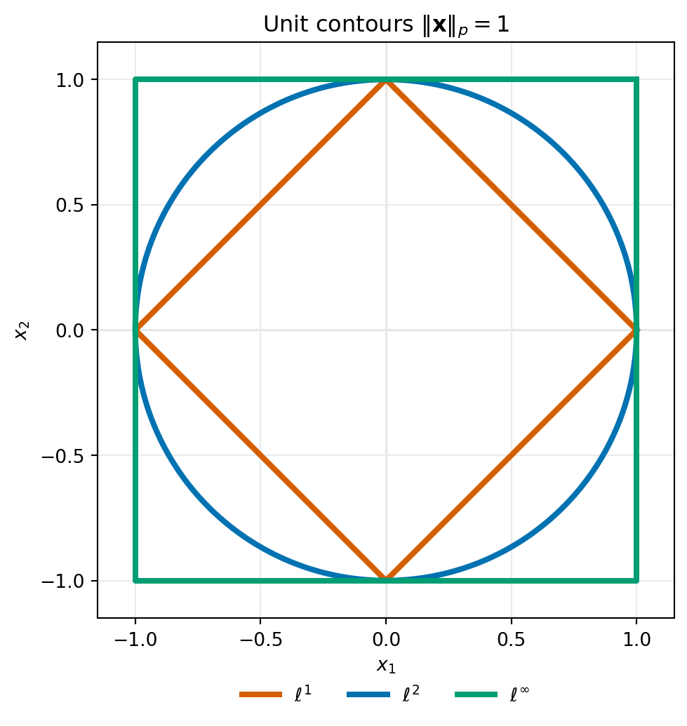
Beyond \(\ell^2\) there is a whole family of \(\ell^p\) norms, each highlighting different structure.
Definition 15 (\(\ell^p\) norms) For \(\bfv \in \Rbb^n\) and \(1 \leq p \leq \infty\): \[
\|\bfv\|_1 = \sum_{i=1}^n |v_i|, \qquad
\|\bfv\|_2 = \left(\sum_{i=1}^n v_i^2\right)^{1/2}, \qquad
\|\bfv\|_\infty = \max_{1 \leq i \leq n} |v_i|.
\] All three are norms on \(\Rbb^n\).
The \(\ell^2\) norm is the only \(\ell^p\) norm induced by an inner product. The \(\ell^1\) and \(\ell^\infty\) norms do not satisfy the parallelogram law \(\|\bfu+\bfv\|^2 + \|\bfu-\bfv\|^2 = 2\|\bfu\|^2 + 2\|\bfv\|^2\), which characterizes inner-product norms.
The most important inequality relating the inner product to the norm is Cauchy–Schwarz.
Theorem 4 (Cauchy–Schwarz inequality) For any \(\bfu, \bfv \in \Rbb^n\), \[
|\langle \bfu, \bfv \rangle| \leq \|\bfu\|\,\|\bfv\|,
\] with equality if and only if \(\bfu\) and \(\bfv\) are proportional (i.e., \(\bfu = c\bfv\) for some \(c \in \Rbb\), or one of them is \(\mathbf{0}\)).
NoteProof
Proof. If \(\bfv = \mathbf{0}\) both sides are zero. Otherwise, for any \(t \in \Rbb\), \[
0 \leq \|\bfu - t\bfv\|^2 = \|\bfu\|^2 - 2t\langle\bfu,\bfv\rangle + t^2\|\bfv\|^2.
\] Minimizing the right-hand side over \(t\) by setting \(t^* = \langle\bfu,\bfv\rangle/\|\bfv\|^2\) gives \[
0 \leq \|\bfu\|^2 - \frac{\langle\bfu,\bfv\rangle^2}{\|\bfv\|^2},
\] which rearranges to the desired inequality. Equality holds iff \(\|\bfu - t^*\bfv\|^2 = 0\), i.e., \(\bfu = t^*\bfv\).
Theorem 4 allows us to define the angle between two nonzero vectors.
Definition 16 (Angle and cosine similarity) For nonzero \(\bfu, \bfv \in \Rbb^n\), Cauchy–Schwarz guarantees \(-1 \leq \dfrac{\langle \bfu,\bfv \rangle}{\|\bfu\|\|\bfv\|} \leq 1\). The angle\(\theta \in [0, \pi]\) between \(\bfu\) and \(\bfv\) is defined by \[
\cos\theta = \frac{\langle \bfu, \bfv \rangle}{\|\bfu\|\,\|\bfv\|}.
\] The quantity \(\cos\theta\) is called the cosine similarity of \(\bfu\) and \(\bfv\).
Example 6 (Cosine similarity in information retrieval) In information retrieval, documents are often represented as TF-IDF vectors \(\bfd \in \Rbb^n\) (one component per vocabulary word). Rather than comparing raw dot products, which favor long documents, one uses the cosine similarity \[
\mathrm{sim}(\bfd_1, \bfd_2) = \frac{\bfd_1^\top \bfd_2}{\|\bfd_1\|_2\,\|\bfd_2\|_2} \in [-1, 1].
\] A value near \(1\) means the documents discuss similar topics; near \(0\) means they are unrelated. The normalization by \(\|\bfd\|\) removes the effect of document length, making a two-sentence abstract and a ten-page paper on the same topic equally similar to a query.
Definition 17 (Orthogonality) Vectors \(\bfu, \bfv \in \Rbb^n\) are orthogonal, written \(\bfu \perp \bfv\), if \(\langle \bfu, \bfv \rangle = 0\). A set of vectors \(\{\bfq_1, ..., \bfq_k\}\) is:
orthogonal if \(\langle \bfq_i, \bfq_j \rangle = 0\) for all \(i \neq j\);
orthonormal if additionally \(\|\bfq_i\|_2 = 1\) for all \(i\).
A basis \(\{\bfq_1, ..., \bfq_n\}\) for \(\Rbb^n\) that is orthonormal is called an orthonormal basis (ONB).
Proposition 1 (Orthogonal sets are linearly independent) Any orthogonal set of nonzero vectors is linearly independent.
NoteProof
Proof. Suppose \(\sum_i c_i \bfq_i = \mathbf{0}\). Taking the inner product with \(\bfq_j\) gives \(c_j \|\bfq_j\|^2 = 0\), so \(c_j = 0\) for all \(j\).
Definition 18 (Orthogonal projection) Let \(S \subseteq \Rbb^n\) be a subspace with orthonormal basis \(\{\bfq_1, ..., \bfq_k\}\). The orthogonal projection of \(\bfv \in \Rbb^n\) onto \(S\) is \[
\mathrm{proj}_S(\bfv)
= \sum_{i=1}^k \langle \bfv, \bfq_i \rangle\, \bfq_i
= \bfQ\bfQ^\top \bfv,
\] where \(\bfQ = [\bfq_1 \mid \cdots \mid \bfq_k] \in \Rbb^{n \times k}\). The matrix \(\bfP = \bfQ\bfQ^\top \in \Rbb^{n \times n}\) is the projection matrix onto \(S\).
Theorem 5 (Properties of projection matrices) Let \(\bfP = \bfQ\bfQ^\top\) be the orthogonal projection onto a subspace \(S\). Then:
Idempotence: \(\bfP^2 = \bfP\).
Symmetry: \(\bfP^\top = \bfP\).
Minimality: \(\mathrm{proj}_S(\bfv)\) is the unique closest point in \(S\) to \(\bfv\), i.e., \[
\mathrm{proj}_S(\bfv) = \argmin_{\bfs \in S} \|\bfv - \bfs\|_2.
\]
Write \(\bfv = \bfP\bfv + (\bfv - \bfP\bfv)\). For any \(\bfs \in S\), \(\|\bfv - \bfs\|^2 = \|\bfP\bfv - \bfs\|^2 + \|\bfv - \bfP\bfv\|^2\) (by (iv) proved next), so the minimum over \(S\) is attained at \(\bfs = \bfP\bfv\).
For any \(\bfq_j\), \(\langle \bfv - \bfP\bfv, \bfq_j \rangle = \langle \bfv, \bfq_j \rangle - \bfq_j^\top\bfQ\bfQ^\top\bfv = \langle\bfv,\bfq_j\rangle - \langle\bfv,\bfq_j\rangle = 0\), so the residual is orthogonal to all basis vectors of \(S\).
TipRemark
Remark. Properties (i) and (ii) together characterize orthogonal projections: any matrix \(\bfP\) satisfying \(\bfP^2 = \bfP\) and \(\bfP^\top = \bfP\) is the orthogonal projection onto its column space \(\Ccal(\bfP)\).
Theorem 6 (Orthogonality of the fundamental subspaces) The four fundamental subspaces satisfy: \[
\Ccal(\bfA^\top) \perp \Ncal(\bfA) \quad\text{in } \Rbb^n,
\qquad
\Ccal(\bfA) \perp \Ncal(\bfA^\top) \quad\text{in } \Rbb^m,
\] and together they give orthogonal direct-sum decompositions: \[
\Rbb^n = \Ccal(\bfA^\top) \oplus \Ncal(\bfA),
\qquad
\Rbb^m = \Ccal(\bfA) \oplus \Ncal(\bfA^\top).
\]
NoteProof
Proof. If \(\bfA^\top\bfv \in \Ccal(\bfA^\top)\) and \(\bfx \in \Ncal(\bfA)\), then \(\langle \bfA^\top\bfv, \bfx\rangle = \bfv^\top(\bfA\bfx) = \bfv^\top\mathbf{0} = 0\), so the two subspaces are orthogonal. Since \(\dim\Ccal(\bfA^\top) + \dim\Ncal(\bfA) = r + (n-r) = n\) by Theorem 3, they span all of \(\Rbb^n\). The argument in \(\Rbb^m\) is analogous.
4 Spectral Structure: Eigenvalues and Eigenvectors
Definition 19 (Eigenvalue and eigenvector) Let \(\bfA \in \Rbb^{n \times n}\). A scalar \(\lambda \in \Rbb\) is an eigenvalue of \(\bfA\) if there exists a nonzero vector \(\bfv \in \Rbb^n\) such that \[
\bfA\bfv = \lambda\bfv.
\] Such a \(\bfv\) is called an eigenvector of \(\bfA\) corresponding to \(\lambda\). The set of all eigenvectors for \(\lambda\), together with \(\mathbf{0}\), forms a subspace called the eigenspace\(E_\lambda = \ker(\bfA - \lambda\bfI)\). The collection of all eigenvalues is the spectrum of \(\bfA\), written \(\sigma(\bfA)\).
The geometric content is immediate: an eigenvector is a direction that \(\bfA\) does not rotate. It is only stretched (or reflected) by the scalar factor \(\lambda\). A large \(|\lambda|\) means \(\bfA\) amplifies that direction; \(|\lambda| < 1\) means it damps it; \(\lambda = 0\) means \(\bfA\) collapses it entirely.
Proposition 2 (Characteristic polynomial)\(\lambda\) is an eigenvalue of \(\bfA \in \Rbb^{n \times n}\) if and only if \[
p(\lambda) \coloneqq \det(\bfA - \lambda\bfI) = 0.
\] The function \(p(\lambda)\) is a polynomial of degree \(n\) called the characteristic polynomial of \(\bfA\).
NoteProof
Proof. \(\bfA\bfv = \lambda\bfv\) with \(\bfv \neq \mathbf{0}\) is equivalent to \((\bfA - \lambda\bfI)\bfv = \mathbf{0}\) having a nontrivial solution, which happens if and only if \(\bfA - \lambda\bfI\) is singular, i.e., \(\det(\bfA - \lambda\bfI) = 0\).
TipRemark
Remark. Over \(\Rbb\), the characteristic polynomial can have complex roots, meaning some real matrices have no real eigenvalues (e.g., a \(90°\) rotation has \(p(\lambda) = \lambda^2 + 1\)). However, symmetric matrices always have real eigenvalues; this is the content of the Spectral Theorem in Section 4.1.
Definition 20 (Algebraic and geometric multiplicity) The algebraic multiplicity of an eigenvalue \(\lambda\) is its multiplicity as a root of \(p(\lambda)\). The geometric multiplicity is \(\dim\ker(\bfA - \lambda\bfI)\). One always has \(1 \leq \text{geometric multiplicity} \leq \text{algebraic multiplicity}\).
Proposition 3 (Eigenvectors for distinct eigenvalues are linearly independent) If \(\lambda_1, ..., \lambda_k\) are distinct eigenvalues of \(\bfA\) with corresponding eigenvectors \(\bfv_1, ..., \bfv_k\), then \(\{\bfv_1, ..., \bfv_k\}\) is linearly independent.
NoteProof
Proof. By induction on \(k\). For \(k = 1\) the claim is immediate since eigenvectors are nonzero. Suppose it holds for \(k-1\) vectors. Given \(\sum_{i=1}^k c_i \bfv_i = \mathbf{0}\), apply \(\bfA\) to get \(\sum_{i=1}^k c_i \lambda_i \bfv_i = \mathbf{0}\), then subtract \(\lambda_k\) times the original relation: \[
\sum_{i=1}^{k-1} c_i(\lambda_i - \lambda_k)\bfv_i = \mathbf{0}.
\] By the inductive hypothesis, \(c_i(\lambda_i - \lambda_k) = 0\) for each \(i < k\). Since \(\lambda_i \neq \lambda_k\), we get \(c_i = 0\) for \(i < k\), and then \(c_k\bfv_k = \mathbf{0}\) forces \(c_k = 0\).
Definition 21 (Diagonalizability) A matrix \(\bfA \in \Rbb^{n \times n}\) is diagonalizable if there exist an invertible \(\bfP \in \Rbb^{n \times n}\) and a diagonal matrix \(\bfD = \mathrm{diag}(\lambda_1, ..., \lambda_n)\) such that \[
\bfA = \bfP\bfD\bfP^{-1}.
\] The columns of \(\bfP\) are eigenvectors of \(\bfA\), and the diagonal entries of \(\bfD\) are the corresponding eigenvalues.
Theorem 7 (Diagonalizability criterion)\(\bfA \in \Rbb^{n \times n}\) is diagonalizable if and only if the geometric multiplicity of every eigenvalue equals its algebraic multiplicity. In particular, if \(\bfA\) has \(n\) distinct eigenvalues then it is diagonalizable.
NoteProof
Proof. \(\bfA\) is diagonalizable iff it has \(n\) linearly independent eigenvectors (which then form the columns of \(\bfP\)). One can show that eigenspaces for different eigenvalues are independent (by Proposition 3 and its extension), so the total count of linearly independent eigenvectors equals the sum of the geometric multiplicities. This sum equals \(n\) iff each geometric multiplicity equals the corresponding algebraic multiplicity.
TipRemark
Remark. Not every matrix is diagonalizable. A matrix with repeated eigenvalues whose geometric multiplicity is strictly less than the algebraic multiplicity is called defective. The canonical obstruction is the \(2 \times 2\) Jordan block \(\bigl(\begin{smallmatrix}0 & 1 \\ 0 & 0\end{smallmatrix}\bigr)\), which has eigenvalue \(0\) with algebraic multiplicity \(2\) but geometric multiplicity \(1\).
Diagonalizability makes repeated application of a matrix cheap: \(\bfA^k = \bfP\bfD^k\bfP^{-1}\), and \(\bfD^k = \mathrm{diag}(\lambda_1^k, ..., \lambda_n^k)\) costs \(O(n)\).
Example 7 (Markov chains and spectral convergence) A Markov chain on \(n\) states is governed by a transition matrix\(\bfT \in \Rbb^{n \times n}\) with \(T_{ij} \geq 0\) and \(\sum_j T_{ij} = 1\). The distribution \(\bfpi_t^\top\) over states satisfies \(\bfpi_{t+1}^\top = \bfpi_t^\top \bfT\), so \(\bfpi_t^\top = \bfpi_0^\top \bfT^t\). Row-stochastic matrices always have \(\lambda_1 = 1\) as the largest eigenvalue. For an irreducible aperiodic chain, \(|\lambda_2| < 1\) and \(\bfT^t \to \mathbf{1}\bfpi_\infty^\top\) as \(t \to \infty\), where \(\bfpi_\infty^\top \bfT = \bfpi_\infty^\top\) is the stationary distribution. The convergence rate is governed by \(|\lambda_2|^t\): a larger spectral gap\(1 - |\lambda_2|\) means faster mixing, a key quantity in the analysis of MCMC samplers used throughout Bayesian data analysis.
Example 8 (Power method) The power method extracts the eigenvector of \(\bfA\) with the largest eigenvalue in absolute value. Starting from a random \(\bfv^{(0)}\), iterate \[
\bfv^{(t+1)} = \frac{\bfA\bfv^{(t)}}{\|\bfA\bfv^{(t)}\|_2}.
\] If \(\bfA\) is diagonalizable with \(|\lambda_1| > |\lambda_2| \geq \cdots\), the iterates converge to the dominant eigenvector at rate \(|\lambda_2/\lambda_1|^t\). Google’s original PageRank algorithm applies the power method to a modified web-link transition matrix to rank web pages by importance. Randomized algorithms for PCA (used in practice for very large matrices) are also based on this idea.
4.1 Symmetric Matrices and the Spectral Theorem
Symmetric matrices, those satisfying \(\bfA^\top = \bfA\), arise constantly in data science. For example, covariance matrices, kernel (Gram) matrices, and graph Laplacians are all symmetric (we’ll see some of these later). Their special structure forces eigenvalues to be real and eigenvectors to be orthogonal, yielding a decomposition far cleaner than the general case.
Proposition 4 (Symmetric matrices have real eigenvalues) If \(\bfA \in \Rbb^{n \times n}\) is symmetric, then every eigenvalue of \(\bfA\) is real.
NoteProof
Proof. Suppose \(\bfA\bfv = \lambda\bfv\) for \(\bfv \neq \mathbf{0}\), allowing \(\lambda \in \Cbb\) and \(\bfv \in \Cbb^n\). Then \[
\bar\lambda\|\bfv\|^2 = \overline{(\lambda\bfv)}^\top\bfv = \overline{(\bfA\bfv)}^\top\bfv = \bar\bfv^\top\bfA^\top\bfv = \bar\bfv^\top\bfA\bfv = \bar\bfv^\top(\lambda\bfv) = \lambda\|\bfv\|^2.
\] Since \(\|\bfv\|^2 > 0\), we conclude \(\bar\lambda = \lambda\), so \(\lambda \in \Rbb\).
Proposition 5 (Eigenvectors for distinct eigenvalues are orthogonal) If \(\bfA\) is symmetric and \(\bfA\bfv_1 = \lambda_1\bfv_1\), \(\bfA\bfv_2 = \lambda_2\bfv_2\) with \(\lambda_1 \neq \lambda_2\), then \(\bfv_1 \perp \bfv_2\).
NoteProof
Proof. Using symmetry of \(\bfA\): \[
\lambda_1\langle\bfv_1,\bfv_2\rangle = \langle\bfA\bfv_1,\bfv_2\rangle = \langle\bfv_1,\bfA^\top\bfv_2\rangle = \langle\bfv_1,\bfA\bfv_2\rangle = \lambda_2\langle\bfv_1,\bfv_2\rangle.
\] Since \(\lambda_1 \neq \lambda_2\), we have \(\langle\bfv_1,\bfv_2\rangle = 0\).
Theorem 8 (Spectral theorem for symmetric matrices) Every symmetric matrix \(\bfA \in \Rbb^{n \times n}\) is orthogonally diagonalizable. That is, there exists an orthogonal matrix \(\bfQ \in \Rbb^{n \times n}\) (i.e., \(\bfQ^\top\bfQ = \bfQ\bfQ^\top = \bfI\)) and a diagonal matrix \(\Lambda = \mathrm{diag}(\lambda_1, ..., \lambda_n)\) with \(\lambda_1 \geq \cdots \geq \lambda_n\) such that \[
\bfA = \bfQ\Lambda\bfQ^\top = \sum_{i=1}^n \lambda_i \bfq_i\bfq_i^\top,
\] where \(\bfq_1, ..., \bfq_n\) are the columns of \(\bfQ\), forming an orthonormal eigenbasis of \(\Rbb^n\).
NoteProof (sketch)
Proof (sketch). By Proposition 4, \(\bfA\) has at least one real eigenvalue \(\lambda_1\) with unit eigenvector \(\bfq_1\). Let \(W = \bfq_1^\perp\). For any \(\bfw \in W\), \(\langle\bfA\bfw, \bfq_1\rangle = \langle\bfw, \bfA\bfq_1\rangle = \lambda_1\langle\bfw,\bfq_1\rangle = 0\), so \(W\) is \(\bfA\)-invariant. The restriction \(\bfA|_W\) is again symmetric, so by induction on \(n\) it has an orthonormal eigenbasis for \(W\). Combining with \(\bfq_1\) yields the full orthonormal eigenbasis for \(\Rbb^n\).
TipRemark
Remark. The outer-product expansion \(\bfA = \sum_i \lambda_i\bfq_i\bfq_i^\top\) is the spectral decomposition. It lets one apply any function \(f\) to a symmetric matrix by \(f(\bfA) \coloneqq \sum_i f(\lambda_i)\bfq_i\bfq_i^\top\), giving a clean definition of the matrix square root, matrix exponential, matrix logarithm, and pseudoinverse.
Definition 22 (Positive semidefinite and positive definite matrices) A symmetric matrix \(\bfA \in \Rbb^{n \times n}\) is:
Positive semidefinite (PSD), written \(\bfA \succeq \mathbf{0}\), if \(\bfx^\top\bfA\bfx \geq 0\) for all \(\bfx \in \Rbb^n\).
Positive definite (PD), written \(\bfA \succ \mathbf{0}\), if \(\bfx^\top\bfA\bfx > 0\) for all \(\bfx \neq \mathbf{0}\).
The scalar \(\bfx^\top\bfA\bfx\) is called the quadratic form of \(\bfA\) at \(\bfx\).
Theorem 9 (Eigenvalue characterization of PSD and PD) Let \(\bfA\) be symmetric with eigenvalues \(\lambda_1, ..., \lambda_n\). Then:
\(\bfA \succeq \mathbf{0}\) if and only if \(\lambda_i \geq 0\) for all \(i\).
\(\bfA \succ \mathbf{0}\) if and only if \(\lambda_i > 0\) for all \(i\).
NoteProof
Proof. By Theorem 8, write \(\bfA = \bfQ\Lambda\bfQ^\top\) and substitute \(\bfy = \bfQ^\top\bfx\) (a bijection since \(\bfQ\) is orthogonal): \[
\bfx^\top\bfA\bfx = \bfy^\top\Lambda\bfy = \sum_{i=1}^n \lambda_i y_i^2.
\] This weighted sum is \(\geq 0\) for all \(\bfy\) iff every \(\lambda_i \geq 0\), and \(> 0\) for all \(\bfy \neq \mathbf{0}\) iff every \(\lambda_i > 0\).
References
Boyd, Stephen P., and Lieven Vandenberghe. 2018. Introduction to Applied Linear Algebra: Vectors, Matrices, and Least Squares. Cambridge University Press.
Pedregosa, F., G. Varoquaux, A. Gramfort, et al. 2011. “Scikit-Learn: Machine Learning in Python.”Journal of Machine Learning Research 12: 2825–30.
Strang, Gilbert. 2019. Linear Algebra and Learning from Data. Wellesley-Cambridge press.
Ström, Jacob. 2015. Immersive Linear Algebra: The World’s First Linear Algebra Book with Fully Interactive Figures. Immersivemath.