Independence and expectations
Definition 1 (Independent and identically distributed) Random variables are independent when learning the values of some gives no information about the others. For two events \(A\) and \(B\), independence means \[
\Pbb(A\cap B)=\Pbb(A)\Pbb(B).
\] For random variables \(X\) and \(Y\), we require this factorization for every pair of events determined by their respective values: \[
\Pbb(X\in A,\,Y\in B)=\Pbb(X\in A)\Pbb(Y\in B)
\] for all measurable sets \(A,B\subseteq\Rbb\).
Now let \(X_1,\ldots,X_n\) be real-valued random variables defined on the same probability space.
They are mutually independent if, for every nonempty subset \(I\subseteq\{1,\ldots,n\}\) and every choice of measurable sets \(A_i\subseteq\Rbb\), \(i\in I\), \[
\Pbb\!\left(\bigcap_{i\in I}\{X_i\in A_i\}\right)
=\prod_{i\in I}\Pbb(X_i\in A_i).
\] In words, joint probabilities factor for every group of variables. When we say that a collection is independent, we mean mutually independent.
They are pairwise independent if, for every \(i\ne j\) and all measurable sets \(A,B\subseteq\Rbb\), \[
\Pbb(X_i\in A,\,X_j\in B)
=\Pbb(X_i\in A)\Pbb(X_j\in B).
\] This only checks groups of two. Mutual independence implies pairwise independence, but the converse can fail when \(n\ge3\).
The abbreviation i.i.d. means mutually independent and identically distributed. Equivalently, there is a common probability distribution \(\mu\) on \(\Rbb\) such that, for all measurable sets \(A_1,\ldots,A_n\), \[
\Pbb(X_1\in A_1,\ldots,X_n\in A_n)
=\prod_{i=1}^n\mu(A_i).
\] For an infinite sequence, these definitions must hold for every finite subcollection.
Example 1 (Pairwise independence does not imply mutual independence) Let \(X_1\) and \(X_2\) be independent Rademacher variables and set \(X_3=X_1X_2\). The triple \((X_1,X_2,X_3)\) takes the four values \[
(1,1,1),\quad(1,-1,-1),\quad(-1,1,-1),\quad(-1,-1,1)
\] with probability \(1/4\) each. Each variable is Rademacher, and for any \(i\ne j\) and \(a,b\in\{-1,1\}\), \[
\Pbb(X_i=a,X_j=b)=\frac14
=\Pbb(X_i=a)\Pbb(X_j=b).
\] Thus the variables are pairwise independent and identically distributed. However, \[
\Pbb(X_1=1,X_2=1,X_3=1)=\frac14
\ne\frac18=\prod_{i=1}^3\Pbb(X_i=1).
\] They are not mutually independent, so they are not i.i.d. Knowing any two determines the third.
Proposition 1 (Expectations of products) If \(X\) and \(Y\) are independent and \(\Ebb[|X|],\Ebb[|Y|]<\infty\), then \[
\Ebb[XY]=\Ebb[X]\Ebb[Y].
\] Thus, the average of the product equals the product of the averages. More generally, for measurable functions \(g\) and \(h\) with \(\Ebb[|g(X)|],\Ebb[|h(Y)|]<\infty\), \[
\Ebb[g(X)h(Y)]=\Ebb[g(X)]\Ebb[h(Y)].
\]
Proof. We’ll show the subcase concerning discrete \(X\) and \(Y\). \[
\begin{aligned}
\Ebb[XY]
&=\sum_x\sum_y xy\,\Pbb(X=x,Y=y) \\
&=\sum_x\sum_y xy\,\Pbb(X=x)\Pbb(Y=y) \\
&=\left(\sum_x x\,\Pbb(X=x)\right)
\left(\sum_y y\,\Pbb(Y=y)\right)
=\Ebb[X]\Ebb[Y].
\end{aligned}
\] Independence is used in the second equality.
Variance
Definition 2 (Variance and standard deviation) The variance of \(X\) is the average squared distance from its mean: \[
\Var(X)
=
\Ebb[(X-\Ebb[X])^2].
\] Its standard deviation is \[
\sigma(X)=\sqrt{\Var(X)}.
\]
The useful computational identity \[
\Var(X)=\Ebb[X^2]-\Ebb[X]^2
\] follows by expanding the square and using linearity of expectation.
For constants \(a,b\in\Rbb\), \[
\Var(aX+b)=a^2\Var(X).
\] Adding a constant moves the center without changing the spread; multiplying by \(a\) scales squared deviations by \(a^2\).
Example 2 (Variance of a Bernoulli variable) If \(X\) is Bernoulli with parameter \(p\), then \(X^2=X\). Therefore \[
\Var(X)
=
\Ebb[X^2]-\Ebb[X]^2
=
p-p^2
=
p(1-p).
\] This is largest when \(p=1/2\) and small when the outcome is nearly certain.
Definition 3 (Covariance) The covariance of \(X\) and \(Y\) is \[
\Cov(X,Y)
=
\Ebb[(X-\Ebb[X])(Y-\Ebb[Y])].
\] Positive covariance means that \(X\) and \(Y\) tend to be above their means together, while negative covariance means that one tends to be high when the other is low.
For two random variables, \[
\Var(X+Y)
=
\Var(X)+\Var(Y)+2\Cov(X,Y).
\] Independent random variables have covariance \(0\), so their variances add. Note: The converse is not generally true! Covariance \(0\) does not by itself imply independence.
Covariance will reappear later as a matrix that describes the directions in which a point cloud varies. For now, its essential role is to show exactly where independence enters the averaging calculation.
Proposition 2 (Averaging away independent noise) Suppose \(X_1,\ldots,X_n\) are independent, each with mean \(\mu\) and variance \(\sigma^2\). Then \[
\Var(\overline{X})
=
\Var\!\left(\frac1n\sum_{i=1}^nX_i\right)
=
\frac1{n^2}\sum_{i=1}^n\Var(X_i)
=
\frac{\sigma^2}{n}.
\] Consequently, \[
\sigma(\overline{X})=\frac{\sigma}{\sqrt n}.
\]
Averaging \(n\) independent measurements reduces the variance by a factor of \(n\) and the standard deviation by a factor of \(\sqrt n\).
Enough of This, Time for Some Cool Stuff
The reason we have building up these probability tools, is because they give us the language to describe a certain phenomena about high dimensional data. Particularly, things in high dimensions are concentrated. The concentration result specifically we’ll get back to toward the end of the course.
But, right now, we can show something illustrative! The approximate Carathéodory theorem tells us that, to approximate a point to a given tolerance, the ‘size of our model’ is independent of both the number of data points and the dimensionality of the data. This is intuition to one the (informal) fundamental theorems of data science!
Theorem 1 (Law of the Lazy Data Scientist) Solving problems exactly is hard. Solving approximate problems approximately can be much easier.
Carathéodory’s theorem: exact and approximate
Definition 4 (Convex hull) Let \(\mathcal{V}=\{\bfv_1,\ldots,\bfv_n\}\subseteq\Rbb^d\) be a set of vectors. A convex combination of its points is a vector of the form \[
\sum_{i=1}^n \alpha_i\bfv_i,
\qquad
\alpha_i\geq 0,
\qquad
\sum_{i=1}^n\alpha_i=1.
\] The convex hull of \(\mathcal{V}\) is the set of all such convex combinations: \[
\operatorname{conv}(\mathcal{V})
=
\left\{
\sum_{i=1}^n\alpha_i\bfv_i
:
\alpha_i\geq 0\text{ for every }i,
\ \sum_{i=1}^n\alpha_i=1
\right\}.
\]
Suppose a point \(\bfx\) belongs to \(\operatorname{conv}(\mathcal{V})\). A natural question you might ask is: how many vectors does it take to represent \(\bfx\) as a convex combination?
At first, it may appear that representing \(\bfx\) requires all \(n\) points. Let’s consult our knowledge of linear algebra to understand why. Put the vectors into the columns of a matrix \(V=[\bfv_1\ \cdots\ \bfv_n]\). Finding a convex representation amounts to solving \[
\begin{bmatrix}V\\ \mathbf{1}^{\mathsf T}\end{bmatrix}\boldsymbol{\alpha}
=
\begin{bmatrix}\bfx\\ 1\end{bmatrix},
\qquad \boldsymbol{\alpha}\geq 0.
\] If the augmented columns \((\bfv_i,1)\) are linearly independent, then these coefficients are unique. Thus, if every coefficient in this unique solution is positive, none of the \(n\) vectors can be omitted. This makes \(n\) a reasonable naive guess.
However, Carathéodory’s theorem says that the ambient dimension, rather than the size of the point cloud, controls how many points are actually needed.
Theorem 2 (Carathéodory’s theorem) Let \(\mathcal{V}\subseteq\Rbb^d\) and let \(\bfx\in\operatorname{conv}(\mathcal{V})\). Then \(\bfx\) is a convex combination of at most \(d+1\) points of \(\mathcal{V}\).
We won’t prove this, but you can see it by inspecting the rank of the matrix we wrote above.
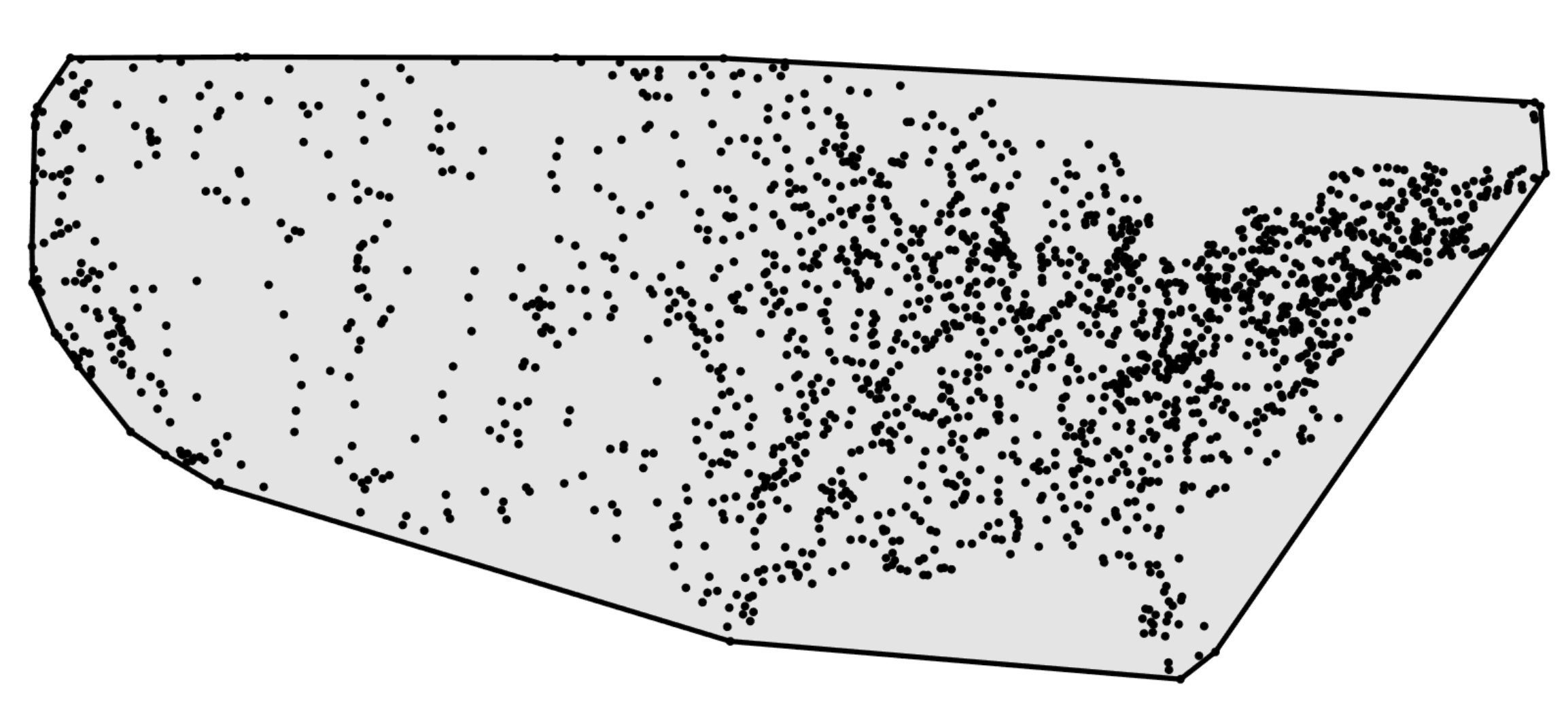
This, on its own, is quite powerful! An exact convex representation needs no more than \(d+1\) points, even if \(\mathcal{V}\) contains millions of them. So for the map of US cities above, I only need three points to represent any of the other cities; despite there being hundreds of points on there.
But when \(d\) is itself enormous, as it can be for images or documents, the bound \(d+1\) may still be too large. If we permit a small error, probability gives a bound that does not involve \(d\) at all.
Theorem 3 (Approximate Carathéodory theorem) Let \(\mathcal{V}=\{\bfv_1,\ldots,\bfv_n\}\subseteq\Rbb^d\) satisfy \(\|\bfv_i\|_2\leq R\) for every \(i\), and let \(\bfx\in\operatorname{conv}(\mathcal{V})\). For every positive integer \(k\), there are \(k\) points \(\bfu_1,\ldots,\bfu_k\in\mathcal{V}\), possibly with repetitions, such that \[
\left\|
\bfx-\frac1k\sum_{j=1}^k\bfu_j
\right\|_2
\leq \frac{R}{\sqrt{k}}.
\] Consequently, for every \(\epsilon>0\), there is a convex combination of at most \[
\max\left\{1,\left\lceil\frac{R^2}{\epsilon^2}\right\rceil\right\}
\] points of \(\mathcal{V}\) whose Euclidean distance from \(\bfx\) is at most \(\epsilon\).
Proof. Because \(\bfx\in\operatorname{conv}(\mathcal{V})\), choose non-negative weights \(\alpha_1,\ldots,\alpha_n\) whose sum is \(1\) and for which \[
\bfx=\sum_{i=1}^n\alpha_i\bfv_i.
\] Define a random vector \(\bfX\) by sampling from this convex combination: \[
\Pbb(\bfX=\bfv_i)=\alpha_i.
\] Then \(\Ebb[\bfX]=\bfx\). Take \(k\) independent copies \(\bfX_1,\ldots,\bfX_k\) of \(\bfX\) and form their average \[
\hat{\bfx}=\frac1k\sum_{j=1}^k\bfX_j.
\] Every possible value of \(\hat{\bfx}\) is an average of \(k\) points from \(\mathcal{V}\). Moreover, independence and \(\Ebb[\bfX_j-\bfx]=\mathbf{0}\) make all of the cross terms vanish. Indeed, if \(j\neq \ell\), then \[
\Ebb\left[
\left\langle \bfX_j-\bfx,\bfX_\ell-\bfx\right\rangle
\right]
=
\left\langle
\Ebb[\bfX_j-\bfx],\Ebb[\bfX_\ell-\bfx]
\right\rangle
=0.
\] It follows that \[
\begin{aligned}
\Ebb\left[\|\hat{\bfx}-\bfx\|_2^2\right]
&=\frac{1}{k^2}
\Ebb\left[
\left\|\sum_{j=1}^k(\bfX_j-\bfx)\right\|_2^2
\right] \\
&=\frac{1}{k}\Ebb\left[\|\bfX-\bfx\|_2^2\right] \\
&=\frac{1}{k}\left(
\Ebb\left[\|\bfX\|_2^2\right]-\|\bfx\|_2^2
\right) \\
&\leq\frac{R^2}{k}.
\end{aligned}
\] The squared error is non-negative, so at least one outcome is no larger than its expectation. For that outcome, \(\|\hat{\bfx}-\bfx\|_2\leq R/\sqrt{k}\). Fixing it proves the first claim. Taking \(k=\max\{1,\lceil R^2/\epsilon^2\rceil\}\) proves the second.
For example, if the data are normalized so that \(R=1\), then \(100\) points suffice for error \(0.1\) whether the ambient dimension is \(100\), \(10{,}000\), or one million.
Thus a high-dimensional convex representation can contain substantial redundancy. Once a controlled amount of error is acceptable, a simple random sampling argument produces a sparse approximation whose size is controlled by the desired accuracy, not by the ambient dimension.