Python for Data Analysis

This course is about the mathematical structure behind data analysis. We will explore that, computationally, with Python because it lets us move back and forth between that mathematics and concrete computations with very little friction. The notation in can be quite close to the linear algebra notation in the notes, the surrounding ecosystem is mature, and the same tools used for small classroom examples also scale to real data sets. While Python is not the point of the course, but it is an important working language for modern applied mathematics, statistics, and machine learning.

The links below are optional references. They are useful if you want a second explanation of Python syntax, a more systematic introduction to programming, or more background on the data-analysis libraries we will use.

Think Python is a gentler, more complete introduction to programming in Python.
A Whirlwind Tour of Python is a compact review of Python syntax and conventions, especially useful if you have programmed before but are new to Python.
Python for Data Analysis gives more depth on the data-analysis stack, especially NumPy and pandas.

Below is a brief taste of how use the language.

NumPy and SciPy: Why Not Plain Python?

Python’s built-in lists are flexible but slow for numerical work. A Python list is a collection of objects, each carrying type information, reference counts, and heap allocations. A loop over ten million numbers can mean ten million Python object touches, very slow.

NumPy solves this by storing data in contiguous blocks of memory (think a C array) and implements operations in compiled C/Fortran under the hood. It’s, therefore, far faster. Moreover, it has a syntax designed to make numerical, mathematical work easier. This is why the computational math ecosystem, in python, is largely standardized around libraries like NumPy.

import numpy as np
from time import perf_counter

n = 5_000_000

# Python list version
py_list = list(range(n))
t0 = perf_counter()
py_sum = sum(x**2 for x in py_list)
t_py = perf_counter() - t0

# NumPy version
np_arr = np.arange(n, dtype=np.float64)
t0 = perf_counter()
np_sum = np.dot(np_arr, np_arr)
t_np = perf_counter() - t0

print(f"Python list : {t_py:.3f} s")
print(f"NumPy array : {t_np:.4f} s")
print(f"Speedup     : {t_py / t_np:.0f}×")

Python list : 0.233 s
NumPy array : 0.0021 s
Speedup     : 113×

This is a ridiculous example, but it’s just to demonstrate the per-operation gains.

Likewise, as mentioned, NumPy also gives you the mental model that matches the math. Arrays are vectors and matrices, and the operations (@ for matrix multiplication, .T for transpose, np.linalg.* for decompositions) map directly onto the notation from math.

A = np.array([[1, 2], [3, 4], [5, 6]])   # 3×2 matrix
v = np.array([1, -1])                     # vector in R^2

print("A @ v =", A @ v)                  # matrix-vector product
print("A.T shape:", A.T.shape)            # transpose: 2×3

A @ v = [-1 -1 -1]
A.T shape: (2, 3)

SciPy sits on top of NumPy and provides higher-level scientific algorithms, e.g. sparse matrix formats, numerical integration, optimization, signal processing, and more. For this course the most relevant piece is scipy.linalg (which exposes LAPACK routines for decompositions not in NumPy). We may reach for SciPy when NumPy’s linalg module is not enough.

scikit-learn

scikit-learn is the standard Python library for classical machine learning. It provides:

A uniform estimator API: every model has .fit(X, y), .predict(X), and .score(X, y).
A large collection of algorithms (linear models, trees, SVMs, clustering, …).
Preprocessing utilities (scalers, encoders, imputers).
Model selection tools (cross-validation, hyperparameter search).
A set of built-in toy datasets for teaching and benchmarking.

We will use scikit-learn heavily throughout the course.

import sklearn
print("scikit-learn version:", sklearn.__version__)

scikit-learn version: 1.8.0

Three Toy Datasets

Iris

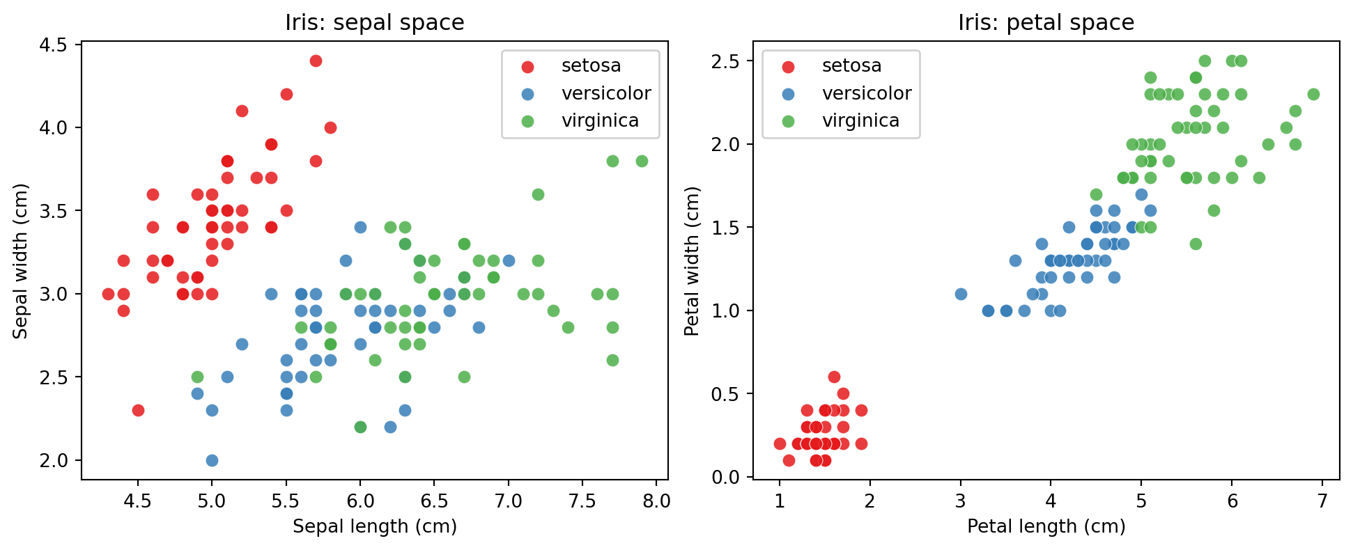
The Iris dataset (Fisher, 1936) records four measurements, sepal length, sepal width, petal length, petal width, for 150 iris flowers spanning three species.

from sklearn.datasets import load_iris

iris = load_iris()
X_iris, y_iris = iris.data, iris.target

print("Shape         :", X_iris.shape)          # (150, 4)
print("Feature names :", iris.feature_names)
print("Classes       :", iris.target_names)
print("Samples/class :", np.bincount(y_iris))

Shape         : (150, 4)
Feature names : ['sepal length (cm)', 'sepal width (cm)', 'petal length (cm)', 'petal width (cm)']
Classes       : ['setosa' 'versicolor' 'virginica']
Samples/class : [50 50 50]

import matplotlib.pyplot as plt
import matplotlib.patches as mpatches

colors = ["#e41a1c", "#377eb8", "#4daf4a"]
labels = iris.target_names

fig, axes = plt.subplots(1, 2, figsize=(10, 4), layout="constrained")

# Sepal space
ax = axes[0]
for k, (c, lbl) in enumerate(zip(colors, labels)):
    mask = y_iris == k
    ax.scatter(X_iris[mask, 0], X_iris[mask, 1], c=c, label=lbl,
               edgecolors="white", linewidths=0.4, s=50, alpha=0.85)
ax.set_xlabel("Sepal length (cm)")
ax.set_ylabel("Sepal width (cm)")
ax.set_title("Iris: sepal space")
ax.legend(framealpha=0.9)

# Petal space
ax = axes[1]
for k, (c, lbl) in enumerate(zip(colors, labels)):
    mask = y_iris == k
    ax.scatter(X_iris[mask, 2], X_iris[mask, 3], c=c, label=lbl,
               edgecolors="white", linewidths=0.4, s=50, alpha=0.85)
ax.set_xlabel("Petal length (cm)")
ax.set_ylabel("Petal width (cm)")
ax.set_title("Iris: petal space")
ax.legend(framealpha=0.9)

plt.show()

Wine

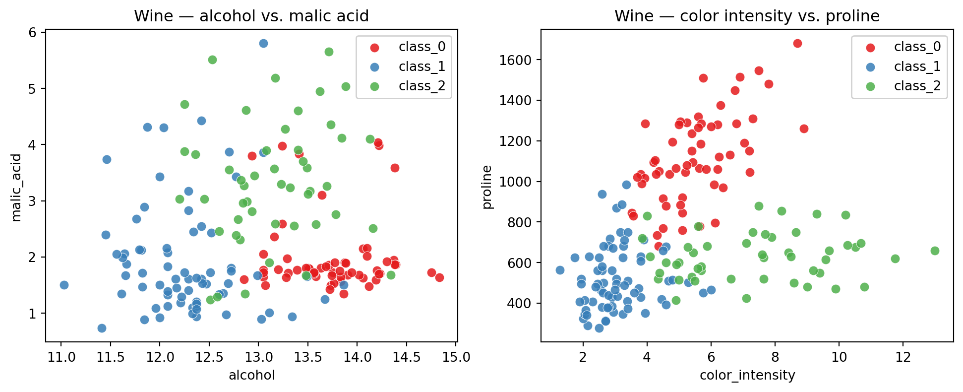
The Wine dataset contains 13 chemical measurements (alcohol content, malic acid, hue, …) for 178 wines from three Italian cultivars.

from sklearn.datasets import load_wine

wine = load_wine()
X_wine, y_wine = wine.data, wine.target

print("Shape         :", X_wine.shape)
print("Feature names :", wine.feature_names)
print("Classes       :", wine.target_names)
print("Samples/class :", np.bincount(y_wine))

Shape         : (178, 13)
Feature names : ['alcohol', 'malic_acid', 'ash', 'alcalinity_of_ash', 'magnesium', 'total_phenols', 'flavanoids', 'nonflavanoid_phenols', 'proanthocyanins', 'color_intensity', 'hue', 'od280/od315_of_diluted_wines', 'proline']
Classes       : ['class_0' 'class_1' 'class_2']
Samples/class : [59 71 48]

fig, axes = plt.subplots(1, 2, figsize=(10, 4), layout="constrained")

feat_pairs = [(0, 1), (9, 12)]   # (alcohol, malic acid) and (color_intensity, proline)
xlabels = [wine.feature_names[i] for i, _ in feat_pairs]
ylabels = [wine.feature_names[j] for _, j in feat_pairs]

for ax, (i, j), xl, yl in zip(axes, feat_pairs, xlabels, ylabels):
    for k, (c, lbl) in enumerate(zip(colors, wine.target_names)):
        mask = y_wine == k
        ax.scatter(X_wine[mask, i], X_wine[mask, j], c=c, label=lbl,
                   edgecolors="white", linewidths=0.4, s=50, alpha=0.85)
    ax.set_xlabel(xl)
    ax.set_ylabel(yl)
    ax.legend(framealpha=0.9)

axes[0].set_title("Wine — alcohol vs. malic acid")
axes[1].set_title("Wine — color intensity vs. proline")
plt.show()

Diabetes

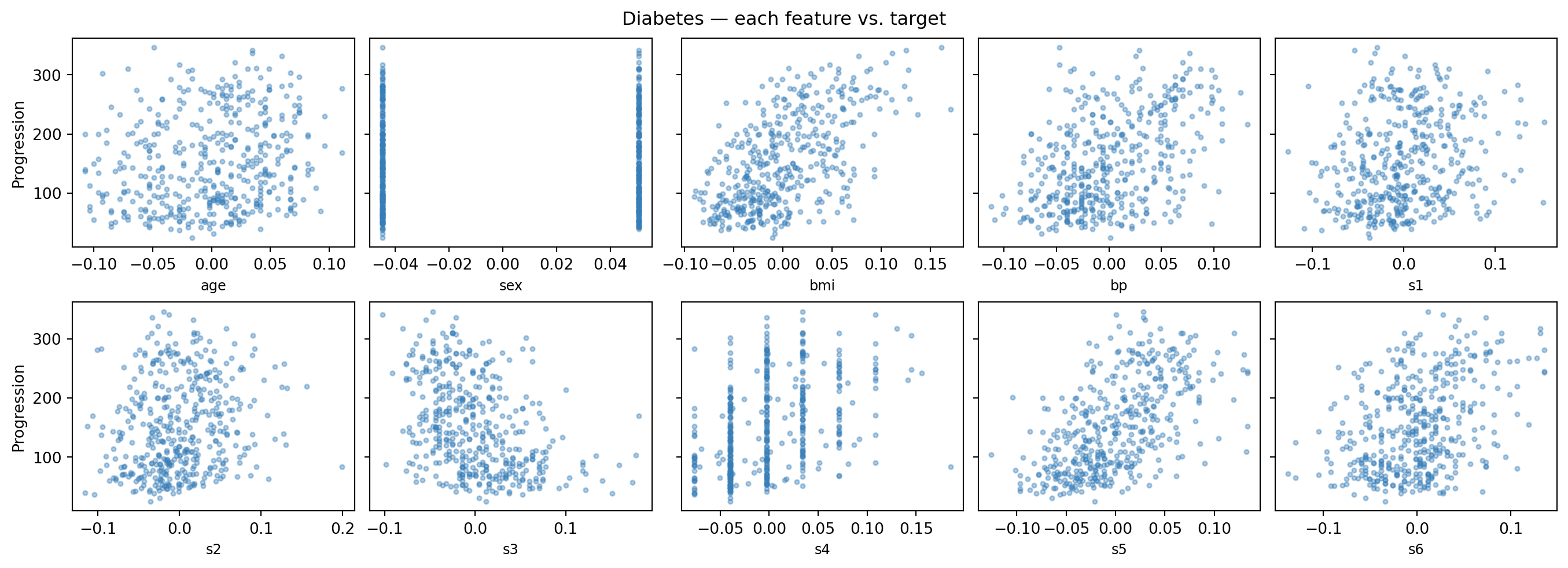
Ten standardized features, 442 patients, one continuous target (disease progression). This is often our canonical small regression benchmark.

from sklearn.datasets import load_diabetes

diabetes = load_diabetes()
X_diab, y_diab = diabetes.data, diabetes.target

print("Shape  :", X_diab.shape)
print("Target : min={:.1f}, max={:.1f}, mean={:.1f}".format(
    y_diab.min(), y_diab.max(), y_diab.mean()))

Shape  : (442, 10)
Target : min=25.0, max=346.0, mean=152.1

fig, axes = plt.subplots(2, 5, figsize=(14, 5), sharey=True, layout="constrained")
axes = axes.ravel()

for i, ax in enumerate(axes):
    ax.scatter(X_diab[:, i], y_diab, s=8, alpha=0.4, color="#377eb8")
    ax.set_xlabel(diabetes.feature_names[i], fontsize=9)
    if i % 5 == 0:
        ax.set_ylabel("Progression")

fig.suptitle("Diabetes — each feature vs. target")
plt.show()