Maximum Mean Discrepancy: Comparing Distributions with Kernels
math
statistics
machine learning
Published
June 22, 2026
I’ve recently had need to understand metrics assessing quality in some generative modeling research I’ve been involved in. One such metric is the Maximum Mean Discrepany (MMD). The best way to understand something is to write and/or teach it, so here it goes.
Broadly speaking, we want to understand a way to measure how different two probability distributions are using only samples. That is, we want a scalar quantity which answers the question
Do samples from model distribution \(Q\) look like samples from target distribution \(P\)?
Fundamentals
Suppose we have two distributions \(P\) and \(Q\) over some space \(\mathcal{X}\). The idea is to try and understand the average behavior of both distributions under some rich family of test functions. For any test function \(f\), we can compare the two expectations
If these expectations differ for some meaningful function \(f\), then \(P\) and \(Q\) are different. We formulate the MMD by seeking the function \(f\) that separates the two distributions the most: \[
\operatorname{MMD}(P, Q)
=
\sup_{\lVert f \rVert_\mathcal{H} \le 1}
\left(
\mathbb{E}_{X \sim P}[f(X)]
-
\mathbb{E}_{Y \sim Q}[f(Y)]
\right).
\]
Here \(\mathcal{H}\) is a reproducing kernel Hilbert space (RKHS), i.e. a function space defined by a positive definite kernel \(k(x, y)\) which measures similarity between two points.
NoteRemark (The Gaussian/RBF Kernel)
Remark (The Gaussian/RBF Kernel). The Gaussian/RBF kernel is \[
k(x, y) = \exp\left(-\frac{\lVert x - y \rVert^2}{2\sigma^2}\right).
\]
This kernel is close to 1 when \(x\) and \(y\) are close, and close to 0 when they are far apart. The bandwidth \(\sigma\) controls what “close” means.
Using this, we can write an alternative, attractice, definition of the MMD. Let’s first define a kernel mean embedding, \[
\mu_P(\cdot) = \mathbb{E}_{X \sim P}[k(X, \cdot)].
\]
This is the average feature representation of samples from \(P\). It can be shown that the MMD is the distance between these two embeddings: \[
\operatorname{MMD}(P, Q) = \lVert \mu_P - \mu_Q \rVert_\mathcal{H}.
\]
Proposition 1 Let \(\mathcal{H}\) be a real RKHS with reproducing kernel \(k\). Assume the kernel mean embeddings \[
\mu_P = \mathbb{E}_{X \sim P}[k(X, \cdot)],
\qquad
\mu_Q = \mathbb{E}_{Y \sim Q}[k(Y, \cdot)]
\] exist as elements of \(\mathcal{H}\). Then \[
\sup_{\lVert f \rVert_\mathcal{H} \le 1}
\left(
\mathbb{E}_{X \sim P}[f(X)]
-
\mathbb{E}_{Y \sim Q}[f(Y)]
\right)
=
\lVert \mu_P - \mu_Q \rVert_\mathcal{H}.
\]
NoteProof
Proof. The defining property of an RKHS is the reproducing property: for every \(f \in \mathcal{H}\) and every point \(x\), \[
f(x) = \langle f, k(x, \cdot) \rangle_\mathcal{H}.
\]
The second equality uses linearity of the inner product and the definition of the mean embedding. So the original MMD definition is \[
\sup_{\lVert f \rVert_\mathcal{H} \le 1}
\langle f, \mu_P - \mu_Q \rangle_\mathcal{H}.
\]
Let \(g = \mu_P - \mu_Q\). For any \(f\) with \(\lVert f \rVert_\mathcal{H} \le 1\), Cauchy-Schwarz gives \[
\langle f, g \rangle_\mathcal{H}
\le
\lvert \langle f, g \rangle_\mathcal{H} \rvert
\le
\lVert f \rVert_\mathcal{H}\lVert g \rVert_\mathcal{H}
\le
\lVert g \rVert_\mathcal{H}.
\] Thus the supremum is at most \(\lVert g \rVert_\mathcal{H}\).
If \(g \ne 0\), choose \[
f =
\frac{g}{\lVert g \rVert_\mathcal{H}}.
\] Then \(\lVert f \rVert_\mathcal{H} = 1\), so this is an allowed test function, and \[
\langle f, g \rangle_\mathcal{H}
=
\left\langle \frac{g}{\lVert g \rVert_\mathcal{H}}, g \right\rangle_\mathcal{H}
=
\lVert g \rVert_\mathcal{H}.
\] So the upper bound is achieved. If \(g = 0\), then \(\langle f, g \rangle_\mathcal{H} = 0\) for every \(f\), and the supremum is also \(0 = \lVert g \rVert_\mathcal{H}\). Therefore the supremum definition and the distance-between-mean-embeddings definition are the same quantity. \(\square\)
For characteristic kernels such as the Gaussian RBF kernel, this distance is zero if and only if the two distributions are the same. That is why MMD can be used as a distribution-level discrepancy, not just a comparison of means in the original data space.
I’ve skipped a lot of details, mainly regarding assumptions, existance, and other technicalities. I refer the interested reading back to (Gretton et al. 2012) for these.
As an additional note, computationally, the following representation of the squared MMD is often attractive.
Proposition 2 The squared MMD has the expectation form \[
\operatorname{MMD}^2(P, Q)
=
\mathbb{E}_{X, X' \sim P}[k(X, X')]
+
\mathbb{E}_{Y, Y' \sim Q}[k(Y, Y')]
-
2\mathbb{E}_{X \sim P, Y \sim Q}[k(X, Y)].
\] where \(X'\) is an independent copy of \(X\) and \(Y'\) is an independent copy of \(Y\).
Substituting these three identities into the squared norm expansion proves the formula. \(\square\)
A Tiny Numerical Example
Let’s compare two tiny one-dimensional sample sets: \[
X = \{0, 1, 2\},
\qquad
Y = \{0, 1, 3\}.
\]
The two sets share two points, but \(Y\) has a point at 3 where \(X\) has a point at 2. We will use an RBF kernel with \(\sigma = 1\).
Code
import numpy as npimport matplotlib.pyplot as pltfrom sklearn.metrics.pairwise import euclidean_distances, rbf_kernelnp.set_printoptions(precision=3, suppress=True)X = np.array([[0.0], [1.0], [2.0]])Y = np.array([[0.0], [1.0], [3.0]])sigma =1.0def rbf_kernel_matrix(a, b, sigma): gamma =1/ (2* sigma**2)return rbf_kernel(a, b, gamma=gamma)Kxx = rbf_kernel_matrix(X, X, sigma)Kyy = rbf_kernel_matrix(Y, Y, sigma)Kxy = rbf_kernel_matrix(X, Y, sigma)print("Kxx: similarities within X")print(Kxx)print("\nKyy: similarities within Y")print(Kyy)print("\nKxy: similarities between X and Y")print(Kxy)
Kxx: similarities within X
[[1.    0.607 0.135]
 [0.607 1.    0.607]
 [0.135 0.607 1.   ]]

Kyy: similarities within Y
[[1.    0.607 0.011]
 [0.607 1.    0.135]
 [0.011 0.135 1.   ]]

Kxy: similarities between X and Y
[[1.    0.607 0.011]
 [0.607 1.    0.135]
 [0.135 0.607 0.607]]
The diagonal entries are 1 because every point is exactly similar to itself. The off-diagonal entries decay as points get farther apart.
The simplest empirical estimate includes all entries of these kernel matrices: \[
\widehat{\operatorname{MMD}}^2_{\text{biased}}
=
\frac{1}{m^2}\sum_{i=1}^m\sum_{j=1}^m k(x_i, x_j)
+
\frac{1}{n^2}\sum_{i=1}^n\sum_{j=1}^n k(y_i, y_j)
-
\frac{2}{mn}\sum_{i=1}^m\sum_{j=1}^n k(x_i, y_j).
\]
It is called the biased estimator because it includes the diagonal self-similarities \(k(x_i, x_i)\) and \(k(y_i, y_i)\). It is still useful and is always nonnegative up to floating point roundoff.
Code
def mmd2_biased(x, y, sigma): kxx = rbf_kernel_matrix(x, x, sigma) kyy = rbf_kernel_matrix(y, y, sigma) kxy = rbf_kernel_matrix(x, y, sigma)return kxx.mean() + kyy.mean() -2* kxy.mean()mmd2 = mmd2_biased(X, Y, sigma)print(f"biased MMD^2 = {mmd2:.6f}")print(f"biased MMD = {np.sqrt(mmd2):.6f}")
biased MMD^2 = 0.087438
biased MMD   = 0.295699
For this example the value is small but not zero. That matches the data: the samples mostly agree, but one point moved from 2 to 3.
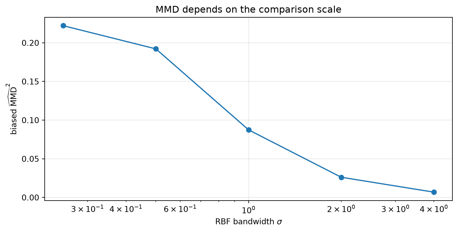
The Impact of Bandwidth
MMD depends on both the samples and the kernel. The RBF bandwidth \(\sigma\) determines the scale at which we compare the distributions.
If \(\sigma\) is very small, then only nearly identical points count as similar. If \(\sigma\) is very large, then almost every point looks similar to every other point and the discrepancy can get washed out.
Code
sigmas = np.array([0.25, 0.5, 1.0, 2.0, 4.0])values = np.array([mmd2_biased(X, Y, s) for s in sigmas])for s, v inzip(sigmas, values):print(f"sigma={s:>4}: biased MMD^2={v:.6f}")
fig, ax = plt.subplots(figsize=(8,4),layout="constrained")ax.plot(sigmas, values, marker="o")ax.set_xscale("log")ax.set_xlabel(r"RBF bandwidth $\sigma$")ax.set_ylabel(r"biased $\widehat{\mathrm{MMD}}^2$")ax.set_title("MMD depends on the comparison scale")ax.grid(True, alpha=0.3)plt.show()
There is no universally correct bandwidth. In practice, people often use the median pairwise distance heuristic, average several RBF kernels with different bandwidths, or tune the bandwidth for the application.
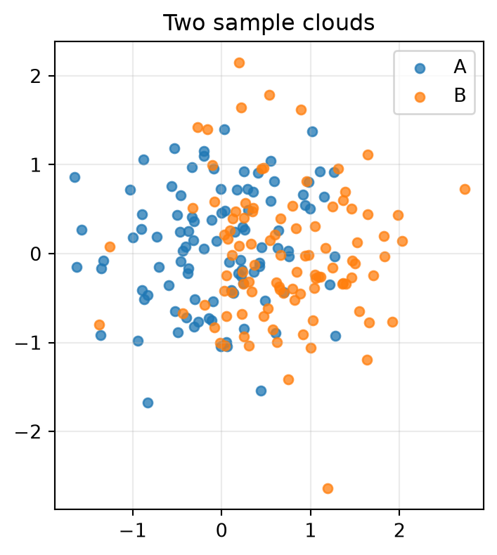
A Slightly Bigger Comparison
Now compare two small 2D sample clouds. The first cloud is centered near \((0, 0)\) and the second is shifted to the right. MMD should be small when we compare the cloud with itself and larger when we compare the original cloud with the shifted one.
The self-comparison is exactly zero for the biased estimator because the same sample set appears on both sides. The shifted comparison is positive because the two clouds have different locations, which changes their kernel mean embeddings.
Biased vs. Unbiased Estimates
There is also an unbiased estimator: \[
\widehat{\operatorname{MMD}}^2_{\text{unbiased}}
=
\frac{1}{m(m-1)}\sum_{i \ne j} k(x_i, x_j)
+
\frac{1}{n(n-1)}\sum_{i \ne j} k(y_i, y_j)
-
\frac{2}{mn}\sum_{i=1}^m\sum_{j=1}^n k(x_i, y_j).
\]
This removes the diagonal self-similarities. It is unbiased as an estimate of the population \(\operatorname{MMD}^2\), but for finite samples it can be slightly negative because it is no longer a squared norm exactly.
Code
def off_diagonal_mean(k): n = k.shape[0]return (k.sum() - np.trace(k)) / (n * (n -1))def mmd2_unbiased(x, y, sigma): kxx = rbf_kernel_matrix(x, x, sigma) kyy = rbf_kernel_matrix(y, y, sigma) kxy = rbf_kernel_matrix(x, y, sigma)return off_diagonal_mean(kxx) + off_diagonal_mean(kyy) -2* kxy.mean()print(f"biased tiny example = {mmd2_biased(X, Y, sigma):.6f}")print(f"unbiased tiny example = {mmd2_unbiased(X, Y, sigma):.6f}")print(f"biased A vs B = {mmd2_biased(A, B, median_sigma):.6f}")print(f"unbiased A vs B = {mmd2_unbiased(A, B, median_sigma):.6f}")
biased tiny example   = 0.087438
unbiased tiny example = -0.345743
biased A vs B         = 0.145871
unbiased A vs B       = 0.138175
For optimization objectives, the biased estimator is often convenient because it behaves like a squared distance. For statistical testing, the unbiased estimator and permutation/bootstrap procedures are often more appropriate.
Optimized JAX Implementation
The sklearn implementation above is a clear baseline implementation. It builds three kernel matrices using rbf_kernel and then averages them. However, if you had to implement this outside of numpy, say in JAX, it’s worth thinking about what an optimized implementation would look like.
There are two useful JAX implementations, with different tradeoffs. The most direct implementation uses nested vmap over a scalar squared-distance function. This computes the distance as written, using the literal \((x - y)^2\) computation.
Code
from time import perf_counterimport jaximport jax.numpy as jnpdef squared_distance_direct(x, y):return jnp.sum((x - y) **2)pairwise_squared_distances_vmap = jax.vmap( jax.vmap(squared_distance_direct, in_axes=(None, 0)), in_axes=(0, None),)def rbf_mean_jax_vmap(x, y, sigma): squared_distances = pairwise_squared_distances_vmap(x, y)return jnp.mean(jnp.exp(-squared_distances / (2* sigma**2)))@jax.jitdef mmd2_biased_jax_vmap(x, y, sigma):return ( rbf_mean_jax_vmap(x, x, sigma)+ rbf_mean_jax_vmap(y, y, sigma)-2* rbf_mean_jax_vmap(x, y, sigma) )
def rbf_mean_jax_gram(x, y, sigma): x2 = jnp.sum(x * x, axis=1, keepdims=True) y2 = jnp.sum(y * y, axis=1, keepdims=True).T squared_distances = jnp.maximum(x2 + y2 -2* (x @ y.T), 0.0)return jnp.mean(jnp.exp(-squared_distances / (2* sigma**2)))@jax.jitdef mmd2_biased_jax_gram(x, y, sigma):return ( rbf_mean_jax_gram(x, x, sigma)+ rbf_mean_jax_gram(y, y, sigma)-2* rbf_mean_jax_gram(x, y, sigma) )
This can be far faster!
Here’s a small benchmark against the sklearn version. Note, scikit-learn is actually implementing the Gram verion above. The benchmark checks that the implementations produce the same biased MMD estimate on a fixed synthetic two-sample problem, then compares their median wall-clock runtime (post-JAX compilation).
Show timing helper
def timed(f): jax.block_until_ready(f()) t = perf_counter() v = jax.block_until_ready(f())return v, perf_counter() - tdef median_timed(f, repeats=7): value =None seconds = []for _ inrange(repeats): value, elapsed = timed(f) seconds.append(elapsed)return value, float(np.median(seconds))
JAX device       = cpu:0
sample shape     = (2000, 16)
sklearn MMD^2    = 0.00887656
JAX Gram MMD^2   = 0.00887656
JAX vmap MMD^2   = 0.00887656
sklearn time     = 81.66 ms
JAX Gram time    = 15.26 ms
JAX vmap time    = 86.29 ms
Gram speedup     = 5.35x
vmap speedup     = 0.95x
The Gram version is usually the fastest of these dense implementations. However, as discussed in this JAX thread on pairwise distances, the Gram version can be numerically unstable when the true distance is small relative to the absolute coordinate values. For example consider two points which are distance \(\sqrt{2}\) apart with a large absolute offset. The direct computation sees the distance, while the Gram calculation loses it.
Gram squared distance   = 0.0
direct squared distance = 2.0
JAX Gram RBF            = 1.00000000
JAX direct RBF          = 0.36787945
The same issue can change the MMD itself. Below, X_edge and Y_edge are not the same point cloud, but the unstable implementations make many cross-similarities look like self-similarities.
Practically speaking, that means that I would likely reach for the naive implementation until convinced that the MMD itself is a bottleneck. Alternatively, one could consider centering the data before the computation, as Euclidean distances are translation-invariant but the floating point cancellation in the Gram identity is not.
With that being said, one can construct estimators of the MMD by considering statistically principled subsamplings of the dataset. This is essentially the concentration of the back half of the paper (Gretton et al. 2012).
References
Gretton, Arthur, Karsten M. Borgwardt, Malte J. Rasch, Bernhard Schölkopf, and Alexander Smola. 2012. “A Kernel Two-Sample Test.”Journal of Machine Learning Research 13 (25): 723–73. https://jmlr.csail.mit.edu/papers/v13/gretton12a.html.